Sea Monsters that Lost their Way

geospatial

machine learning

textual analysis

Predicting uncertain species of cetacean strandings recorded by the Natural History Museum

Author

Carl Goodwin

Published

December 4, 2021

Modified

June 29, 2024

The Natural History Museum began recording cetacean (whales, dolphins and porpoises) strandings in 1913 (Natural History Museum 2019). Let’s explore this 1913-1989 dataset.

library(conflicted)
library(tidyverse)
conflict_prefer_all("dplyr", quiet = TRUE)
library(tidymodels)
library(probably)
library(finetune)
library(textrecipes)
library(stopwords)
library(clock)
library(glue)
library(janitor)
library(vip)
conflicts_prefer(vip::vi)
library(tictoc)
library(patchwork)
library(future)
library(paletteer)
library(ggfoundry)
library(usedthese)

conflict_scout()

plan(multisession, workers = 10)

theme_set(theme_bw())


pal_name <- "wesanderson::Darjeeling2"

pal <- paletteer_d(pal_name)

display_palette(pal, pal_name)

strandings_df <- read_csv("strandings.csv", show_col_types = FALSE) |>
  clean_names() |> 
  mutate(
    date_rep = date_parse(date, format = "%d/%m/%Y"),
    length = parse_number(length_et),
    species_lumped = fct_lump_n(species, 20),
    across(ends_with("_val"), as.integer),
    rep_comment = comment
  )

# glimpse(strandings_df)

Exploratory

Some of the species labels contain a question mark or forward slash. This indicates uncertainty, so it might be fun to see if a machine learning model (multi-class classification) could learn from the known species and suggest an appropriate species where it’s uncertain.

strandings_df2 <- 
  strandings_df |> 
  mutate(species_uncertainty =
      if_else(str_detect(species, "[?/]"), "Uncertain", "Known"))

strandings_df2 |> 
  filter(species_uncertainty == "Uncertain") |> 
  count(species, sort = TRUE, name = "Count") |> 
  slice_head(n = 6)

species	Count
delphis/coeruleoalba	48
phocoena?	42
melaena?	20
delphis?	18
truncatus?	18
acutorostrata?	12

The date variable has many NA’s. Fortunately, the components to construct many of these are in the year_val, month_val and day_val variables. With a little wrangling and imputation, we can coalesce these variables into a new date. This will be useful since plots of sample species by year, month and week of stranding suggest a de-constructed date could be a useful predictor.

strandings_df2 |> 
  select(date_rep, year_val, month_val, day_val) |> 
  summary()

    date_rep             year_val      month_val         day_val     
 Min.   :1913-02-13   Min.   :   0   Min.   : 0.000   Min.   : 0.00  
 1st Qu.:1933-09-09   1st Qu.:1933   1st Qu.: 4.000   1st Qu.: 9.00  
 Median :1954-04-13   Median :1955   Median : 7.000   Median :16.00  
 Mean   :1955-01-08   Mean   :1954   Mean   : 6.766   Mean   :15.66  
 3rd Qu.:1979-03-21   3rd Qu.:1979   3rd Qu.:10.000   3rd Qu.:22.00  
 Max.   :1989-12-25   Max.   :1989   Max.   :12.000   Max.   :31.00  
 NA's   :121

strandings_df3 <- strandings_df2 |>
  mutate(
    month_val = if_else(month_val == 0, mean(month_val) |> 
                          as.integer(), month_val),
    day_val = if_else(day_val == 0, mean(day_val) |> as.integer(), day_val),
    day_val = if_else(day_val == 0, 1L, day_val),
    date2 = date_build(year_val, month_val, day_val, invalid = "NA"),
    .by = species
  ) |> 
  mutate(date3 = coalesce(date_rep, date2),
         date_rep = if_else(is.na(date_rep), lag(date3), date3)
         ) |> 
  select(-date2, -date3, -ends_with("_val"))

example_species <-
  c("musculus", "melas", "crassidens", "borealis", "coeruleoalba")

known_species <- strandings_df3 |> 
  filter(species_uncertainty == "Known")

plot_date_feature <- \(var) {
  known_species |>
    mutate(
      year = get_year(date_rep),
      month = get_month(date_rep),
      week = as_iso_year_week_day(date_rep) |> get_week()
    ) |>
    filter(species %in% example_species) |>
    count(species, {{ var }}) |>
    ggplot(aes({{ var }}, species)) +
    geom_violin(
      alpha = 0.7,
      fill = pal[3],
      show.legend = FALSE
    ) +
    labs(
      title = glue("Variation in {str_to_title(as.character(var))}",
                   " of Stranding for Known Species"),
      x = NULL, y = glue("{str_to_title(as.character(var))}")
    )
}

c("year", "month", "week") |> 
  map(sym) |> 
  map(plot_date_feature) |> 
  wrap_plots(ncol = 1)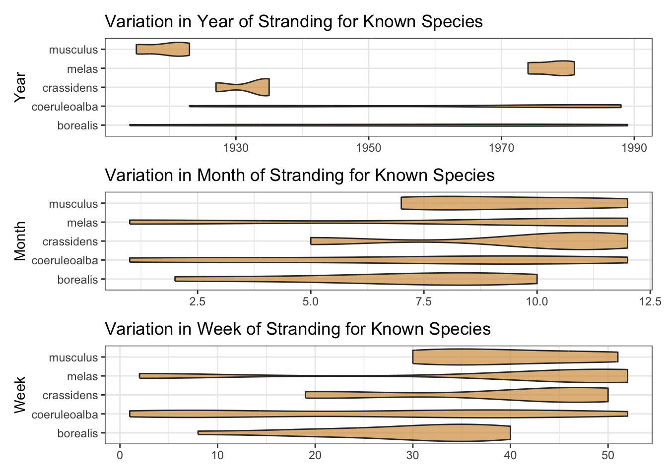

Do latitude and longitude carry useful predictive information?

A geospatial visualisation of strandings shows some species do gravitate towards particular stretches of coastline, e.g. “acutus” and “albirostris” to the east, and “coeruleoalba” to the south-west.

Some species may also be more prone to mass stranding, so something that indicates whether a species has such a history (in these data) may be worth including in the mix.

uki <- map_data("world", region = c("uk", "ireland"))

labels <- c("Mass", "Single")

uki |> 
  ggplot() +
  geom_map(aes(long, lat, map_id = region), map = uki, 
           colour = "black", fill = "grey90", size = 0.1) +
  geom_jitter(aes(longitude, latitude, colour = mass_single, 
                  size = mass_single), 
              alpha = 0.5, data = known_species) +
  facet_wrap(~ species_lumped, nrow = 3) +
  coord_map("mollweide") +
  scale_size_manual(values = c(1, 0.5), labels = labels) +
  scale_colour_manual(values = pal[c(3, 2)], labels = labels) +
  theme_void() +
  theme(legend.position = "top", 
        strip.text = element_text(colour = "grey50")) +
  labs(title = "Strandings by Species", 
       colour = NULL, size = NULL)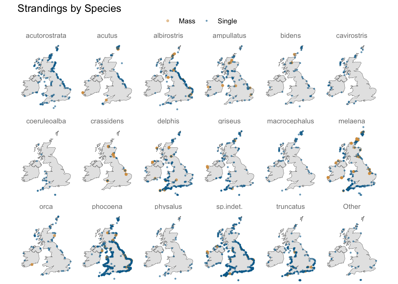

# Add history of mass stranding
strandings_df4 <- strandings_df3 |> 
  mutate(mass_possible = min(mass_single, na.rm = TRUE),
         .by = species)

Some records are missing the length measurement of the mammal. Nonetheless, where present, this is likely to be predictive, and may help, for example, separate species labelled as “delphis/coeruleoalba” where the length is at the extreme ends of the “delphis” range as we see below. And the range of length may differ by mammal sex.

known_species |>
  mutate(sex = case_match(
    sex,
    "M" ~ "Male",
    "F" ~ "Female",
    .default = "Unknown"
  )) |> 
  filter(species_lumped != "Other") |> 
  count(species_lumped, length, sex) |> 
  mutate(species_lumped = fct_reorder(species_lumped, 
                                      desc(length), min, na.rm = TRUE)) |> 
  ggplot(aes(length, species_lumped)) + 
  geom_violin(aes(fill = if_else(str_detect(species_lumped, "^de|^co"), 
                                 TRUE, FALSE)), show.legend = FALSE) +
  facet_wrap(~ sex) +
  scale_fill_manual(values = pal[c(1, 5)]) +
  labs(title = "Variation in Species Length by Sex", 
       x = NULL, y = "Length (metres)")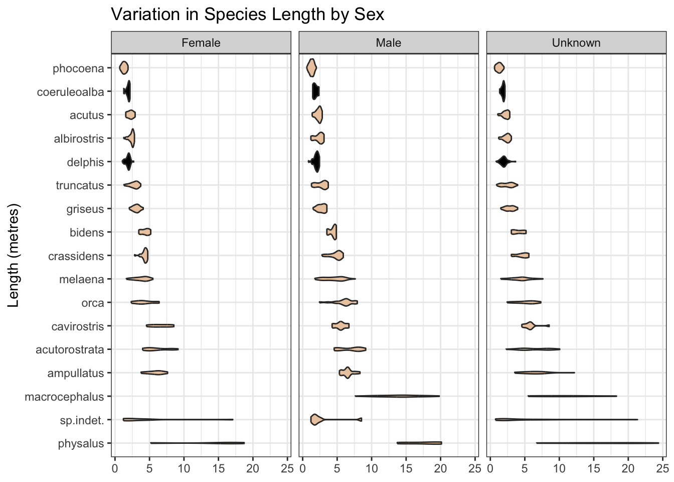

With map coordinates not always available, county could be, with a little string cleaning, a useful additional predictor.

strandings_df4 |> 
  count(county) |> 
  filter(str_detect(county, "Shet|Northumberland")) |> 
  rename(County = county, Count = n)

County	Count
Fair Isle, Shetland Isles	1
Northumberland	89
Northumberland.	1
Shetland Islands, Scotland	232
Shetland Isles, Scotland	35
Shetland, Scotland	1
Shetlands, Scotland	1

regex_pattern <-
  c("[,/].*$",
    "(?<!Che|Hamp|Lanca|North York)-?shire",
    " Isl.*$",
    " &.*$",
    "[-.]$")

strandings_df5 <- strandings_df4 |>
  mutate(
    county = str_remove_all(county, str_c(regex_pattern, collapse = "|")),
    county = recode(
      county,
      "Carnarvon" = "Caernarvon",
      "E.Lothian" = "East Lothian",
      "Shetlands" = "Shetland",
      "W.Glamorgan" = "West Glamorgan",
      "S.Glamorgan" = "South Glamorgan"
    )
  ) 

strandings_df4 |>
  summarise(counties_before = n_distinct(county))

counties_before
146

strandings_df5 |>
  summarise(counties_after = n_distinct(county))

counties_after
109

Whilst count also appears to hold, based on the plot pattern below, species-related information, I’m not going to use it as a predictor as we do not know enough about how it was derived, as reflected in these variable descriptions.

strandings_df5 |>
  ggplot(aes(count, species, colour = species_uncertainty)) +
  geom_jitter(alpha = 0.5, size = 2) +
  scale_x_log10() +
  scale_colour_manual(values = pal[c(1, 5)]) +
  labs(title = "How 'Count' Relates to Species", 
       x = NULL, y = "Count (log10)", colour = "Species") +
  theme(legend.position = "top")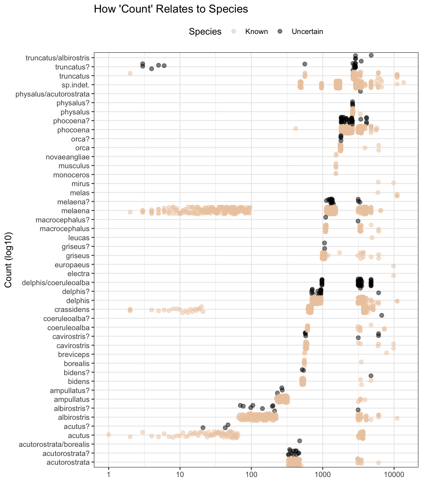

Modelling

So, I’ll set aside the rows where the species is uncertain (to be used later for new predictions), and I’ll train a model on 75% of known species, and test it on the remaining 25%. I’ll use the following predictors:

latitude and longitude
Mammal length and sex
mass_possible indicating a species history of mass strandings
date reported converted into decimal, week, month and year
county may be useful, especially where the longitude and latitude are missing
fam_genus which narrows the range of likely species

I’d like to also make use of the textrecipes(Hvitfeldt 2022) package. I can tokenise the textual information in rep_comment and location to see if these add to the predictive power of the model.

I’ll tune the model using tune_race_anova(Kuhn 2022) which quickly discards hyperparameter combinations showing little early promise.

known_species <- strandings_df5 |>
  filter(species_uncertainty == "Known") |>
  mutate(across(
    c(
      "species",
      "mass_single",
      "mass_possible",
      "county",
      "location",
      "sex",
      "fam_genus"
    ),
    factor
  ))

set.seed(123)

data_split <-
  known_species |>
  mutate(species = fct_drop(species)) |> 
  initial_split(strata = species)

train <- data_split |> training()

test <- data_split |> testing()

predictors <-
  c(
    "latitude",
    "longitude",
    "length",
    "mass_single",
    "mass_possible",
    "county",
    "location",
    "rep_comment",
    "sex",
    "fam_genus"
  )

recipe <-
  train |>
  recipe() |>
  update_role(species, new_role = "outcome") |>
  update_role(all_of(predictors), new_role = "predictor") |>
  update_role(!has_role("outcome") & !has_role("predictor"), 
              new_role = "id") |>
  step_date(date_rep, features = c("decimal", "week", "month", "year"), 
            label = FALSE) |>
  step_tokenize(location, rep_comment) |>
  step_stopwords(location, rep_comment) |>
  step_tokenfilter(location, rep_comment, max_tokens = tune()) |> #100
  step_tf(location, rep_comment) |>
  step_zv(all_predictors()) |>
  step_dummy(all_nominal_predictors())

xgb_model <-
  boost_tree(trees = tune(), # 440
             mtry = tune(), # 0.6
             learn_rate = 0.02) |> 
  set_mode("classification") |>
  set_engine("xgboost", 
             count = FALSE,
             verbosity = 0,
             tree_method = "hist")

xgb_wflow <- workflow() |>
  add_recipe(recipe) |>
  add_model(xgb_model)

set.seed(9)

folds <- vfold_cv(train, strata = species)

set.seed(10)

tic()

tune_result <- xgb_wflow |>
  tune_race_anova(
    resamples = folds,
    grid = crossing(
      trees = seq(200, 520, 40),
      mtry = seq(0.5, 0.7, 0.1),
      max_tokens = seq(80, 120, 20)
      ),
    control = control_race(),
    metrics = metric_set(accuracy)
  )

toc()

119.753 sec elapsed

tune_result |> 
  plot_race() + 
  labs(title = "Early Elimination of Parameter Combinations")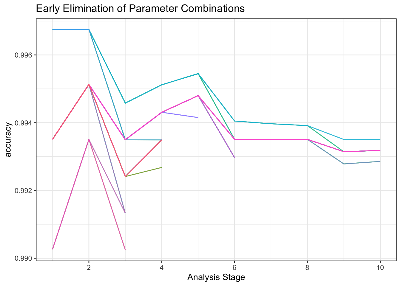

set.seed(123)

xgb_fit <- xgb_wflow |>
  finalize_workflow(tune_result |> 
                      select_best(metric = "accuracy")) |> 
  fit(train)

Having fitted the model with the 3080 records in the training data, I’ll test its accuracy on the 1028 records of known species the model has not yet seen.

Without spending time on alternative models, we’re getting a reasonable result for the “porpoise” of this post, as reflected in both the accuracy metric and confusion matrix.

xgb_results <- xgb_fit |> 
  augment(new_data = test)

xgb_results |>
  accuracy(species, .pred_class)

.metric	.estimator	.estimate
accuracy	multiclass	0.9931907

xgb_results |>
  conf_mat(species, .pred_class) |>
  autoplot(type = "heatmap") +
  scale_fill_gradient2(
    mid = "white",
    high = pal[1],
    midpoint = 0
  ) +
  labs(title = "Confusion Matrix") +
  theme(axis.text.x = element_text(angle = 45, hjust = 1))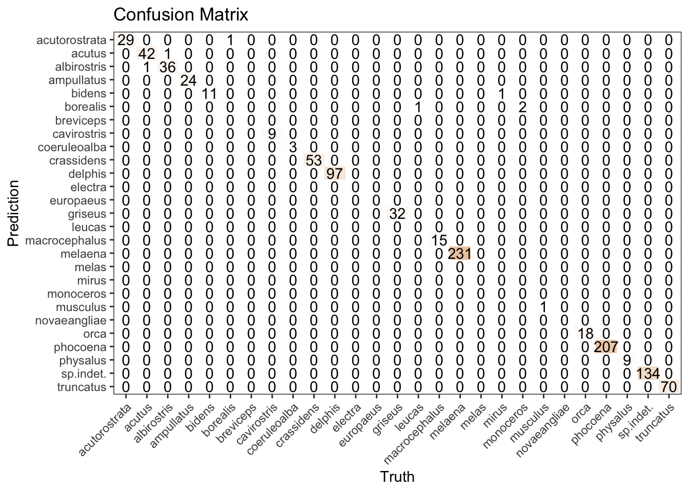

The top variable importance scores include fam_genus, many of the rep_comment tokens, plus length, mass-possible, date_decimal, date_year, and latitude.

vi(xgb_fit |> extract_fit_parsnip()) |> 
  arrange(desc(Importance)) |> 
  mutate(ranking = row_number()) |> 
  slice_head(n = 40)

Variable	Importance	ranking
fam_genus_Phocoena	0.1122588	1
fam_genus_Globicephala	0.1024888	2
tf_rep_comment_unidentified	0.0715584	3
fam_genus_Delphinus	0.0631823	4
tf_rep_comment_false	0.0511217	5
fam_genus_Tursiops	0.0468992	6
fam_genus_Lagenorhynchus	0.0419043	7
fam_genus_Grampus	0.0297059	8
length	0.0284722	9
tf_rep_comment_sided	0.0272743	10
tf_rep_comment_lesser	0.0248649	11
fam_genus_Hyperoodon	0.0230048	12
tf_rep_comment_dolphin	0.0228118	13
tf_rep_comment_beaked	0.0219151	14
fam_genus_Pseudorca	0.0218223	15
tf_rep_comment_bottle	0.0215637	16
tf_rep_comment_porpoise	0.0194644	17
fam_genus_Orcinus	0.0188337	18
tf_rep_comment_long	0.0172326	19
tf_rep_comment_rorqual	0.0161952	20
fam_genus_Physeter	0.0158765	21
tf_rep_comment_finned	0.0156477	22
fam_genus_odontocete	0.0145794	23
tf_rep_comment_common	0.0142945	24
mass_possible_S	0.0135635	25
tf_rep_comment_white	0.0120380	26
fam_genus_Ziphius	0.0116641	27
fam_genus_Mesoplodon	0.0110397	28
tf_rep_comment_fin	0.0105581	29
tf_rep_comment_whale	0.0102145	30
tf_rep_comment_pilot	0.0093067	31
fam_genus_Stenella	0.0087473	32
date_rep_decimal	0.0074321	33
tf_rep_comment_risso’s	0.0069388	34
date_rep_year	0.0067197	35
fam_genus_cetacean	0.0066044	36
tf_rep_comment_sowerby’s	0.0055218	37
tf_rep_comment_nosed	0.0053597	38
tf_rep_comment_cuvier’s	0.0040589	39
tf_rep_comment_sperm	0.0029688	40

Do the predictions look reasonable?

The class probability is spread across 27 species. I’m going to set a high threshold of 0.9, meaning the predicted species needs to be a pretty confident prediction.

xgb_preds <- xgb_fit |> 
  augment(new_data = strandings_df5 |> 
            filter(species_uncertainty == "Uncertain"))

species_levels <- xgb_preds |> 
  select(starts_with(".pred_"), -.pred_class) |> 
  names() |> 
  as.factor()

subset_df <- xgb_preds |>
  mutate(
    .class_pred = make_class_pred(
      .pred_acutorostrata,
      .pred_acutus,
      .pred_albirostris,
      .pred_ampullatus,
      .pred_bidens,
      .pred_borealis,
      .pred_breviceps,
      .pred_cavirostris,
      .pred_coeruleoalba,
      .pred_crassidens,
      .pred_delphis,
      .pred_electra,
      .pred_europaeus,
      .pred_griseus,
      .pred_leucas,
      .pred_macrocephalus,
      .pred_melaena,
      .pred_melas,
      .pred_mirus,
      .pred_monoceros,
      .pred_musculus,
      .pred_novaeangliae,
      .pred_orca,
      .pred_phocoena,
      .pred_physalus,
      .pred_sp.indet.,
      .pred_truncatus,
      levels = levels(species_levels),
      min_prob = .9
    )
  )

subset_df |>
  summarise(n = n(), .by = c(species, .class_pred)) |> 
  arrange(species, desc(n)) |> 
  rename("Actual" = species, "Predicted" = .class_pred, "Count" = n)

Actual	Predicted	Count
acutorostrata/borealis	.pred_acutorostrata	1
acutorostrata?	.pred_acutorostrata	12
acutus?	.pred_acutus	3
albirostris?	.pred_albirostris	9
ampullatus?	.pred_ampullatus	3
bidens?	.pred_bidens	2
bidens?	[EQ]	1
cavirostris?	.pred_cavirostris	7
coeruleoalba?	.pred_coeruleoalba	1
delphis/coeruleoalba	[EQ]	48
delphis?	.pred_delphis	18
griseus?	.pred_griseus	2
macrocephalus?	.pred_macrocephalus	2
melaena?	.pred_melaena	20
orca?	.pred_orca	4
phocoena?	.pred_phocoena	42
physalus/acutorostrata	[EQ]	1
physalus?	.pred_physalus	4
truncatus/albirostris	[EQ]	5
truncatus?	.pred_truncatus	18

The majority of the 203 uncertain records are predicted to be as suspected in the original labelling. The remainder are classed as equivocal as they have not met the high bar of a 0.9-or-above probability for a single species.

R Toolbox

Summarising below the packages and functions used in this post enables me to separately create a toolbox visualisation summarising the usage of packages and functions across all posts.

used_here()

Package	Function
base	as.character[2], as.integer[2], c[13], is.na[1], levels[1], library[17], mean[2], min[1], names[1], seq[3], set.seed[4], summary[1]
clock	as_iso_year_week_day[1], date_build[1], date_parse[1], get_month[1], get_week[1], get_year[1]
conflicted	conflict_prefer_all[1], conflict_scout[1], conflicts_prefer[1]
dplyr	across[2], arrange[2], case_match[1], coalesce[1], count[4], desc[3], filter[7], if_else[6], lag[1], mutate[13], n[1], n_distinct[2], recode[1], rename[2], row_number[1], select[3], slice_head[2], starts_with[1], summarise[3]
finetune	control_race[1], plot_race[1], tune_race_anova[1]
forcats	fct_drop[1], fct_lump_n[1], fct_reorder[1]
future	plan[1]
generics	as.factor[1], augment[2], fit[1]
ggfoundry	display_palette[1]
ggplot2	aes[6], autoplot[1], coord_map[1], element_text[2], facet_wrap[2], geom_jitter[2], geom_map[1], geom_violin[2], ggplot[4], labs[6], map_data[1], scale_colour_manual[2], scale_fill_gradient2[1], scale_fill_manual[1], scale_size_manual[1], scale_x_log10[1], theme[3], theme_bw[1], theme_set[1], theme_void[1]
glue	glue[2]
hardhat	extract_fit_parsnip[1]
janitor	clean_names[1]
paletteer	paletteer_d[1]
parsnip	boost_tree[1], set_engine[1], set_mode[1]
patchwork	wrap_plots[1]
probably	make_class_pred[1]
purrr	map[2]
readr	parse_number[1], read_csv[1]
recipes	all_nominal_predictors[1], all_predictors[1], has_role[2], recipe[1], step_date[1], step_dummy[1], step_zv[1], update_role[3]
rsample	initial_split[1], testing[1], training[1], vfold_cv[1]
stringr	str_c[1], str_detect[3], str_remove_all[1], str_to_title[2]
textrecipes	step_stopwords[1], step_tf[1], step_tokenfilter[1], step_tokenize[1]
tictoc	tic[1], toc[1]
tidyr	crossing[1]
tidyselect	all_of[1], ends_with[2]
tune	finalize_workflow[1], select_best[1], tune[3]
usedthese	used_here[1]
vip	vi[1]
workflows	add_model[1], add_recipe[1], workflow[1]
yardstick	accuracy[1], conf_mat[1], metric_set[1]

References

Hvitfeldt, Emil. 2022. “Textrecipes: Extra ’Recipes’ for Text Processing.” https://CRAN.R-project.org/package=textrecipes.

Kuhn, Max. 2022. “Finetune: Additional Functions for Model Tuning.” https://CRAN.R-project.org/package=finetune.

Natural History Museum. 2019. “Query on the Natural History Museum Data Portal (Data.nhm.ac.uk) (4311 Records).” Natural History Museum. https://doi.org/10.5519/QD.IWG63595.