A Footnote in History

The grammar of tables, footnotes and occupations consigned to history

The nature of employment has seen significant shifts over time. Occupations are being consigned to ‘footnotes in history’ whilst others grow driven by trends such as concern for the environment.

Producing a journal-quality table requires fine-grained and reproducible control over presentation. Surgical targeting of footnotes, capable of adapting to changes in the underlying data, is one example.

This post briefly explores the shifts in the nature of employment whilst at the same time more fully exploring the grammar of tables gt(Iannone et al. 2022): The natural companion to the grammar of graphics ggplot2(Wickham 2016).

library(conflicted)
library(tidyverse)
conflict_prefer_all("dplyr")
library(readxl)
library(gt)
library(usedthese)

conflict_scout()

2 conflicts:
* `filter`: [dplyr]
* `lag`   : [dplyr]

In Digging Deep, the DT package is used to produce a reactable table; one with sortable and searchable columns. DT is intended as an R interface to the DataTables library, but reactivity is not yet supported in gt.

Data frames are liberally printed across all projects including, for example, a table to summarise an auto-generated overview of R packages and functions used in each project. The YAML option df-print: kable renders a nice table (with striped rows) in these cases.

For this project something a little more sophisticated is needed.

As a guiding principle, Posit packages are my first port of call. This provides a confidence in cross-package consistency, interoperability, longevity and an investment in development and support. Hence gt is the go-to package for the footnoted table further down.

As the intent is to present a summary in the style of the Financial Times, we’ll need a suitable custom colour palette.

theme_set(theme_bw())

cols <- c(
  "#FFF1E5", "#F2DFCE",
  "#333333", "#800D33",
  "#C00000", "#00994D"
) |>
  fct_inorder()

tibble(x = 1:6, y = 1) |>
  ggplot(aes(x, y, fill = cols)) +
  geom_col(colour = "white") +
  geom_label(aes(label = cols),
    nudge_y = -0.1, fill = "white"
  ) +
  annotate(
    "label",
    x = 3.5, y = 0.5,
    label = "Financial Times",
    fill = "white",
    alpha = 0.8,
    size = 6
  ) +
  scale_fill_manual(values = as.character(cols)) +
  theme_void() +
  theme(legend.position = "none")

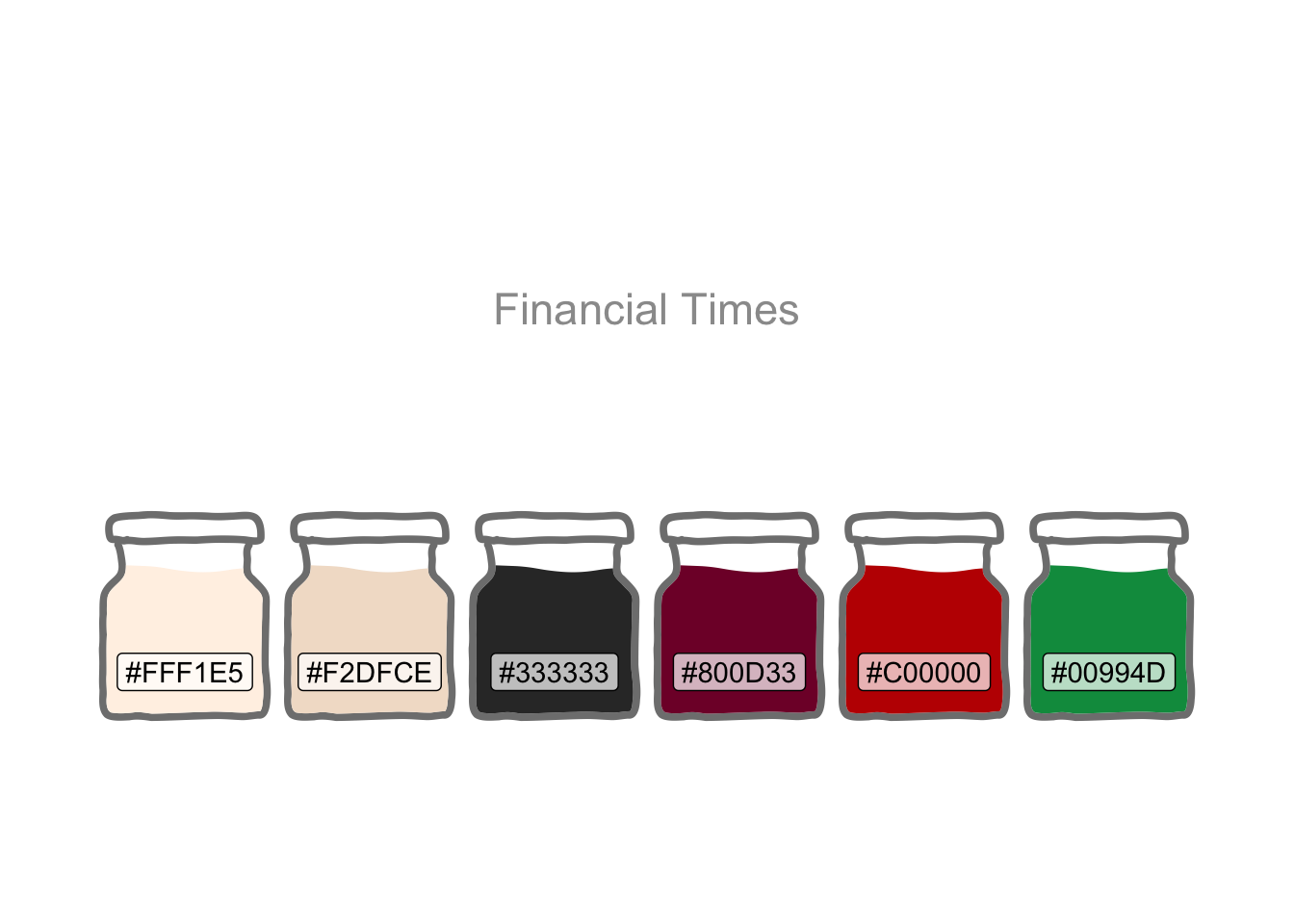
The labour market data are sourced from the Office for National Statistics¹.

read_data <- \(x) {
  read_xlsx(
    x,
    skip = 12,
    col_names = c(
      "occupation",
      "persons"
    ),
    col_types = c(
      "text",
      "numeric",
      "skip",
      "skip",
      "skip",
      "skip",
      "skip"
    )
  )
} |> 
  mutate(year = x |> str_remove(".xlsx") |> as.integer())

pop_df <- list("2004.xlsx", "2021.xlsx") |> 
  map(read_data) |> 
  list_rbind()

There’s a hierarchy to the data, so I’ll extract the lowest level and then slice off the top and bottom occupations based on their percentage change over time.

change_df <- pop_df |> 
  filter(str_starts(occupation, "\\d{4} ")) |> 
  pivot_wider(names_from = year, values_from = persons) |> 
  separate_wider_regex(occupation, 
                       c(soc = "\\d{4}", " ", occupation = ".*")) |> 
  mutate(change = `2021` / `2004` - 1) |> 
  arrange(desc(change)) |> 
  mutate(group = if_else(row_number() <= 10, "Risers", "Fallers")) |> 
  slice(c(1:10, (n()-10):n())) |> 
  relocate(group)

The handling of footnotes is a particularly nice feature in gt: The package automatically assigns, and maintains the order of, the superscripted numbers (could also be symbols) to ensure they flow naturally. And targeting offers a high degree of control and reproducibility.

For example, two entries (highlighted light blue) in the table below use the abbreviation n.e.c.. The footnote may be targeted at rows which contain that string rather than having to manually identify the rows. And once added, any subsequent footnotes would be renumbered to maintain the flow. So, if I were to change the source datasets to different years or countries, all references to n.e.c. would be auto-magically found and appropriately footnoted.

gt_tbl <- change_df |>
  gt(rowname_col = c("occupation"), groupname_col = "group") |>
  tab_header(title = "UK Employment by Occupation") |> 
  tab_options(table.width = pct(100)) |> 
  fmt_number(
    columns = starts_with("2"),
    decimals = 0
  ) |>
  fmt_percent(
    columns = starts_with("c"),
    decimals = 0,
    force_sign = TRUE
  ) |>
  sub_missing() |>
  tab_spanner(
    label = "Year",
    columns = starts_with("2")
  ) |> 
  tab_style(
    style = cell_text(transform = "capitalize"),
    locations = cells_column_labels(!starts_with("s"))
  ) |> 
  tab_style(
    style = cell_text(transform = "uppercase"),
    locations = cells_column_labels("soc")
  ) |> 
  tab_footnote(
    footnote = "Not elsewhere classified",
    locations = cells_stub(rows = contains("n.e.c."))
  ) |> 
  tab_footnote(
    footnote = "Count of all persons",
    locations = cells_column_spanners()
  ) |>
  tab_footnote(
    footnote = "Standard Occupational Classification 2020",
    locations = cells_column_labels(columns = "soc")
  ) |>
  tab_footnote(
    footnote = "Top & bottom 10 occupations ordered by percent change",
    locations = cells_row_groups(groups = c("Risers", "Fallers"))
  ) |>
  tab_footnote(
    footnote = "Figures suppressed as statistically unreliable",
    locations = cells_body(
      columns = c(change, `2021`),
      rows = is.na(change)
    )
  ) |>
  tab_source_note(source_note = "Source: Office for National Statistics (ONS)")

gt_tbl |>
  tab_style_body(
    style = cell_fill(color = "lightblue"),
    pattern = "n.e.c.",
    extents = "stub"
  ) |> 
  opt_stylize(style = 6, color = "gray", add_row_striping = TRUE) |> 
  as_raw_html()

UK Employment by Occupation
	soc2	Year1		change
		2004	2021
Risers3
Industrial cleaning process occupations	9132	26,300	241,100	+817%
Health professionals n.e.c.4	2219	9,000	70,100	+679%
Police community support officers	3315	2,100	13,900	+562%
Business and financial project management professionals	2424	58,300	350,000	+500%
Advertising and public relations directors	1134	19,400	69,000	+256%
IT business analysts, architects and systems designers	2135	82,800	270,500	+227%
Aircraft maintenance and related trades	5235	27,200	88,300	+225%
Quality assurance and regulatory professionals	2462	43,700	138,000	+216%
Officers of non-governmental organisations	4114	41,800	127,200	+204%
Environment professionals	2142	17,500	52,100	+198%
Fallers3
Sheet metal workers	5213	29,100	10,900	−63%
Process operatives n.e.c.4	8119	22,200	8,200	−63%
Footwear and leather working trades	5413	13,000	4,800	−63%
Printing machine assistants	8127	22,600	8,100	−64%
Assemblers (electrical and electronic products)	8131	63,200	20,700	−67%
Printers	5422	63,600	8,900	−86%
Chartered architectural technologists	2435	2,400	5 —	5 —
Moulders, core makers and die casters	5212	3,900	5 —	5 —
Air-conditioning and refrigeration engineers	5225	19,400	5 —	5 —
Pre-press technicians	5421	8,600	5 —	5 —
Coal mine operatives	8122	2,600	5 —	5 —
Source: Office for National Statistics (ONS)
1 Count of all persons
2 Standard Occupational Classification 2020
3 Top & bottom 10 occupations ordered by percent change
4 Not elsewhere classified
5 Figures suppressed as statistically unreliable

The above table uses one of the in-built style theme options. It looks clean and polished. But sometimes the table to be published needs a high degree of customisation to match, for example, a specific branding. gt offers this as we’ll demonstrate by attempting to replicate the style employed by the market data in the Financial Times.

gt_ft <- gt_tbl |> 
  tab_options(
    table.border.top.color = "#FFF1E5",
    table.border.bottom.color = "#FFF1E5",
    table.background.color = "#FFF1E5",
    table.font.size = px(10),
    table.font.color = "#262A33",
    heading.align = "left",
    heading.title.font.size = px(20),
    heading.title.font.weight = "bold",
    heading.background.color = "#FFF1E5",
    row.striping.include_table_body = TRUE,
    row.striping.include_stub = TRUE,
    row.striping.background_color = "#F2DFCE",
    row_group.background.color = "#FFF1E5"
  ) |> 
  tab_header(title = html("UK Employment by Occupation  ", 
                          local_image("logo.png", height = 20))) |> 
  tab_style(
    style = list(
      cell_text(font = "Financier Display"),
      cell_borders(sides = "bottom", weight = px(3), color = "#262A33")
      ),
    locations = cells_title()
  ) |>
  tab_style(
    style = cell_text(size = px(14)),
    locations = cells_row_groups()
  ) |> 
  tab_style(
    style = cell_text(color = "#800D33", weight = "bold"),
    locations = cells_stub()
  ) |> 
  tab_style(
    style = cell_text(weight = "bold"),
    locations = list(cells_column_labels(), 
                     cells_column_spanners(), 
                     cells_row_groups())
  ) |> 
  tab_style(
    style = cell_borders(style = "hidden"),
    locations = list(cells_body(),
                     cells_row_groups(),
                     cells_stub())
  ) |>
  tab_style(
    style = cell_text(color = "#00994D", weight = "bold"),
    locations = cells_body(
      columns = change,
      rows = change >= 0
    )
  ) |> 
  tab_style(
    style = cell_text(color = "#C00000", weight = "bold"),
    locations = cells_body(
      columns = change,
      rows = change < 0
    )
  ) |> 
  tab_style(
    style = cell_text(color = "grey40", size = px(9)),
    locations = list(cells_footnotes(), cells_source_notes())
  )

gt_ft |> as_raw_html()

UK Employment by Occupation
	soc2	Year1		change
		2004	2021
Risers3
Industrial cleaning process occupations	9132	26,300	241,100	+817%
Health professionals n.e.c.4	2219	9,000	70,100	+679%
Police community support officers	3315	2,100	13,900	+562%
Business and financial project management professionals	2424	58,300	350,000	+500%
Advertising and public relations directors	1134	19,400	69,000	+256%
IT business analysts, architects and systems designers	2135	82,800	270,500	+227%
Aircraft maintenance and related trades	5235	27,200	88,300	+225%
Quality assurance and regulatory professionals	2462	43,700	138,000	+216%
Officers of non-governmental organisations	4114	41,800	127,200	+204%
Environment professionals	2142	17,500	52,100	+198%
Fallers3
Sheet metal workers	5213	29,100	10,900	−63%
Process operatives n.e.c.4	8119	22,200	8,200	−63%
Footwear and leather working trades	5413	13,000	4,800	−63%
Printing machine assistants	8127	22,600	8,100	−64%
Assemblers (electrical and electronic products)	8131	63,200	20,700	−67%
Printers	5422	63,600	8,900	−86%
Chartered architectural technologists	2435	2,400	5 —	5 —
Moulders, core makers and die casters	5212	3,900	5 —	5 —
Air-conditioning and refrigeration engineers	5225	19,400	5 —	5 —
Pre-press technicians	5421	8,600	5 —	5 —
Coal mine operatives	8122	2,600	5 —	5 —
Source: Office for National Statistics (ONS)
1 Count of all persons
2 Standard Occupational Classification 2020
3 Top & bottom 10 occupations ordered by percent change
4 Not elsewhere classified
5 Figures suppressed as statistically unreliable

R Toolbox

Summarising below the packages and functions used in this post enables me to separately create a toolbox visualisation summarising the usage of packages and functions across all posts.

used_here()

Package	Function
base	as.character[1], as.integer[1], c[8], is.na[1], library[5], list[5]
conflicted	conflict_prefer_all[1], conflict_scout[1]
dplyr	arrange[1], desc[1], filter[1], if_else[1], mutate[3], n[2], relocate[1], row_number[1], slice[1]
forcats	fct_inorder[1]
ggplot2	aes[2], annotate[1], geom_col[1], geom_label[1], ggplot[1], scale_fill_manual[1], theme[1], theme_bw[1], theme_set[1], theme_void[1]
gt	as_raw_html[2], cell_borders[2], cell_fill[1], cell_text[9], cells_body[4], cells_column_labels[4], cells_column_spanners[2], cells_footnotes[1], cells_row_groups[4], cells_source_notes[1], cells_stub[3], cells_title[1], fmt_number[1], fmt_percent[1], gt[1], html[1], local_image[1], opt_stylize[1], pct[1], px[5], sub_missing[1], tab_footnote[5], tab_header[2], tab_options[2], tab_source_note[1], tab_spanner[1], tab_style[10], tab_style_body[1]
purrr	list_rbind[1], map[1]
readxl	read_xlsx[1]
stringr	str_remove[1], str_starts[1]
tibble	tibble[1]
tidyr	pivot_wider[1], separate_wider_regex[1]
tidyselect	contains[1], starts_with[4]
usedthese	used_here[1]

References

Iannone, Richard, Joe Cheng, Barret Schloerke, Ellis Hughes, and JooYoung Seo. 2022. “Gt: Easily Create Presentation-Ready Display Tables.”

Wickham, Hadley. 2016. “Ggplot2: Elegant Graphics for Data Analysis.” https://ggplot2.tidyverse.org.

Footnotes

1. Contains public sector information licensed under the Open Government Licence v3.0.