Bayes Lived Here (Probably)

bayesian regression

markov chain monte carlo

machine learning

web scraping

special effects

Predicting the interest rate for a fixed-rate mortgage using Bayesian regression

Author

Carl Goodwin

Published

June 12, 2023

Modified

July 5, 2023

It’s quite common in the UK, and London in particular, for prominent individuals, such as Dickens, Darwin and Galton, who passed at least 20 years ago, to be commemorated by a plaque on a building in which they lived or with which they were associated.

Thomas Bayes lived in Tunbridge Wells, a few miles to the north of London. His former home has a plaque on the front gate. I couldn’t resist a little digital graffiti.

Mortgages weren’t a thing back then. So I wonder what he would have made of modelling fixed mortgage interest rates with Bayesian linear regression and tuning tree-based models with Bayesian optimisation.

library(conflicted)
library(tidyverse)
conflict_prefer_all("dplyr", quiet = TRUE)
library(tidymodels)
library(feasts)
library(tsibble)
library(wesanderson)
library(glue)
library(scales)
library(patchwork)
library(ggfx)
library(janitor)
library(rvest)
library(broom.mixed)
library(imputeTS)
library(readxl)
library(rstantools)
library(shapviz)
library(kernelshap)
library(finetune)
library(tictoc)
library(usedthese)

conflict_scout()

theme_set(theme_bw())

cols <- c(
  "#7E1134", "#EDD5C5",
  "#057683", "#F3E2D8",
  "black", "#7F7E7C"
) |>
  fct_inorder()

tibble(x = 1:6, y = 1) |>
  ggplot(aes(x, y, fill = cols)) +
  geom_col(colour = "white") +
  geom_label(aes(label = cols),
    nudge_y = -0.1, fill = "white"
  ) +
  annotate(
    "label",
    x = 3.5, y = 0.5,
    label = "Palette from Feature Image",
    fill = "white",
    alpha = 0.8,
    size = 6
  ) +
  scale_fill_manual(values = as.character(cols)) +
  theme_void() +
  theme(legend.position = "none")

Banks review their mortgage interest rates in response to changes in the central bank rate. Fixed-rate mortgages are further influenced by the value of gilts (government bonds). Banks rely less on the wholesale market to fund mortgages when their balance sheet is well supported by savings made by households.

So, to forecast an average fixed 5-year (75% loan-to-value) mortgage rate (mortgage), I’ll try using the central bank rate (cbr), the 5-year yield from British Government Securities (gilt), the ratio of retail deposits to the value of outstanding mortgages (retail_ratio) and the number of new mortgage approvals (approvals). All sourced from the Bank of England¹.

get_rate <- \(y, z) {
  url <-
    str_c(
      "https://www.bankofengland.co.uk/boeapps/database/",
      "fromshowcolumns.asp?Travel=NIxAZxSUx&FromSeries=1&ToSeries=50&",
      "DAT=ALL&",
      "FNY=Y&CSVF=TT&html.x=66&html.y=26&SeriesCodes=", y,
      "&UsingCodes=Y&Filter=N&title=Quoted%20Rates&VPD=Y"
    )
  
  read_html(url) |>
    html_element("#stats-table") |>
    html_table() |>
    clean_names() |>
    mutate(date = dmy(date)) |> 
    rename({{ z }} := 2)
}

pwalk(
  list(
    x = c("cbr_df", "mor_df", "gil_df", "ret_df", "out_df", "app_df"),
    y = c("IUMBEDR", "IUMBV42", "IUMSNPY", "LPMVRJX", "LPMB3TA", "LPMB3VA"),
    z = c("cbr", "mortgage", "gilt", "retail", "outstanding", "approvals")
  ),
  \(x, y, z) assign(x, get_rate(y, {{ z }}), .GlobalEnv)
)

boe_list <- list(cbr_df, mor_df, gil_df, ret_df, out_df, app_df)

joined_df <- 
  reduce(boe_list, left_join, join_by(date)) |> 
  filter(date <= "2023-04-30") |>
  mutate(retail_ratio = retail / outstanding) |>
  select(-retail, -outstanding)

To enable forecasting to year-end, forward-looking estimates are required for the predictors: cbr², gilt³ and approvals⁴. Imputation is used to linearly interpolate the interim months.

forward_df <- joined_df |>
  rows_append(
    tribble(
      ~date, ~cbr, ~gilt, ~approvals, 
      ymd("2023-06-30"), 4.57, 4.29, 49000, 
      ymd("2023-09-30"), 4.90, NA, NA,
      ymd("2023-12-31"), 4.92, NA, NA,
      ymd("2024-03-31"), 4.64, NA, NA,
      ymd("2024-06-30"), 4.30, 4.92, 68000, 
    )
  )

filled_df <-
  tibble(date = seq(
    joined_df$date |> nth(-2L) |> floor_date("month"),
    forward_df$date |> last() |> floor_date("month"),
    by = "month"
  )) |>
  mutate(date = rollforward(date)) |>
  left_join(forward_df, join_by(date)) |>
  mutate(across(-c(date, mortgage), na_interpolation)) 

forecast_df <-
  bind_rows(actual = joined_df, forecast = filled_df, .id = "id") |>
  arrange(date, id) |>
  distinct(date, .keep_all = TRUE) |>
  mutate(across(c(gilt, cbr),
    list(
      lag1 = lag,
      lag2 = \(x) lag(x, 2),
      lag3 = \(x) lag(x, 3),
      lag12 = \(x) lag(x, 12)
    ),
    .names = "{.col}_{.fn}"
  )) |>
  filter(date >= "1995-01-01", date <= "2023-12-31") |> 
  mutate(mortgage_cut = cut_number(mortgage, 10))

All these historical data and forward-looking estimates may then be visualised to get an overall view.

plot_compare <- \(x){
  forecast_df |>
    ggplot(aes(date, {{ x }}, colour = id)) +
    geom_line() +
    geom_vline(xintercept = ymd("2023-04-30"), linetype = "dashed", colour = "grey60") +
    scale_colour_manual(values = as.character(cols[c(5, 3)])) +
    scale_x_date(date_breaks = "2 years", date_labels = "%Y") +
    scale_y_continuous(labels = label_number(suffix = "%")) +
    labs(x = NULL, colour = NULL) +
    theme(
      axis.text.x = element_blank(),
      axis.ticks.x = element_blank(),
      legend.position = "none"
    )
}

p1 <- plot_compare(cbr) +
  labs(title = "Key Rates", y = "Central\nBank Rate") +
  theme(legend.position = "right")

p2 <- plot_compare(gilt) +
  labs(y = "5-year\nGilt")

p3 <- plot_compare(retail_ratio) +
  scale_y_continuous(labels = label_number()) +
  labs(y = "Retail\nRatio")

p4 <- plot_compare(approvals) +
  scale_y_continuous(labels = label_number()) +
  labs(y = "Approvals")

p5 <- plot_compare(mortgage) +
  labs(y = "Fixed 5-year\nMortgage") +
  theme(
    axis.text.x = element_text(angle = 45, hjust = 1),
    axis.ticks.x = element_line()
  )

p1 / p2 / p3 / p4 / p5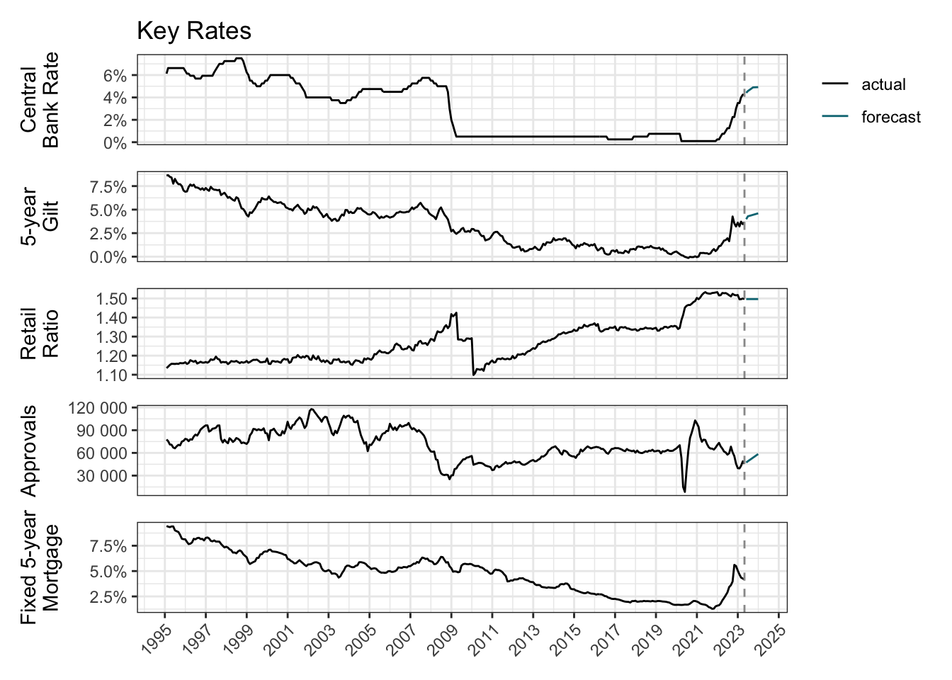

Cross-correlation shows not only the strength of the relationship between the response (mortgage) and explanatory variables, but also highlights any lagged effects. Spikes outside the dashed lines indicate significant correlation beyond “white noise”.

plot_xcorr <- \(x){
  forecast_df |>
    mutate(date = yearmonth(date)) |>
    as_tsibble(index = date) |>
    CCF({{ x }}, mortgage, lag_max = 40) |>
    autoplot() +
    scale_y_continuous(limits = c(-1, 1)) +
    labs(y = NULL) +
    theme(
      axis.text.y = element_blank(),
      axis.ticks.y = element_blank()
    )
}

c1 <- plot_xcorr(cbr) +
  labs(title = "CBR", y = "Cross Correlation") +
  theme_bw()

c2 <- plot_xcorr(gilt) +
  ggtitle("Gilt")

c3 <- plot_xcorr(retail_ratio) +
  ggtitle("Retail Ratio")

c4 <- plot_xcorr(approvals) +
  ggtitle("Approvals")

c1 + c2 + c3 + c4 + 
  plot_layout(nrow = 1) +
  plot_annotation(title = "5-year Fixed-rate Mortgage Correlated With:")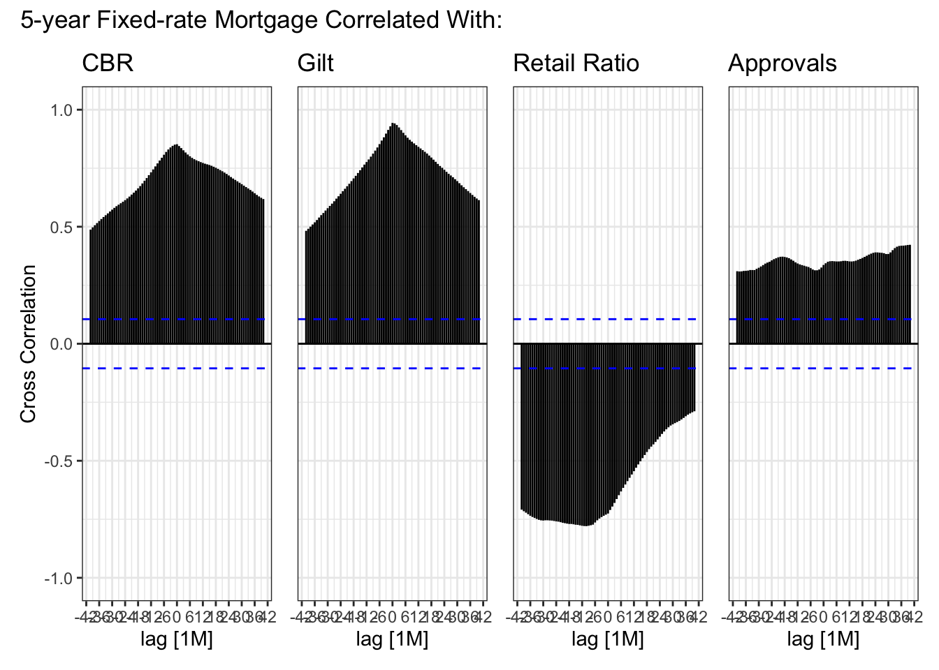

history_df <- forecast_df |>
  filter(id == "actual")

plot_lm <- \(x) {
  history_df |>
    ggplot(aes({{ x }}, mortgage)) +
    geom_point() +
    geom_smooth(method = "lm", colour = cols[3]) +
    scale_x_continuous(labels = label_number(accuracy = 0.1, suffix = "%")) +
    scale_y_continuous(labels = label_number(accuracy = 0.1, suffix = "%")) +
    theme(
      axis.text.y = element_blank(),
      axis.ticks.y = element_blank()
    ) +
  labs(y = NULL)
}

l1 <- plot_lm(cbr) +
  labs(y = "Mortgage") +
  theme_bw()

l2 <- plot_lm(gilt)

l3 <- plot_lm(retail_ratio) +
  scale_x_continuous(labels = label_number(accuracy = 0.1))

l4 <- plot_lm(approvals) +
  scale_x_continuous(
    labels = label_number(
      accuracy = 1,
      scale_cut = cut_short_scale()
    )
  )

l1 + l2 + l3 + l4 + 
  plot_annotation(title = "Independent vs Potential Explanatory Variables") +
  plot_layout(nrow = 1)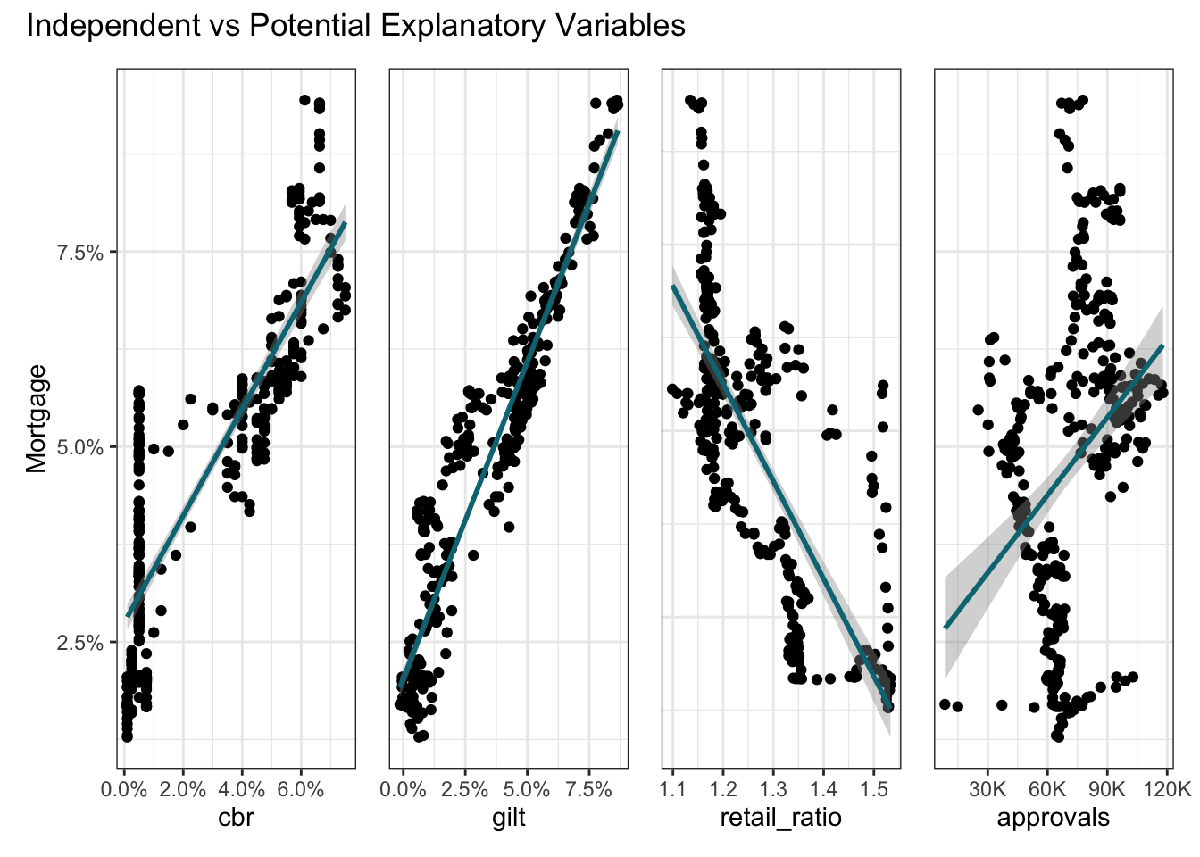

One could try a time series model⁵, e.g. ARIMA. This would focus on patterns and pattern changes in the historical mortgage data, i.e. autocorrelation, seasonality and trend. External regressors like cbr and gilt, could then be additionally used to reduce any remaining unexplained variance. The train/test split would be a time-based split. This kind of statistical technique works well when relationships and trends in the historical data are clear and fairly stable such as, for example, with electricity consumption.

A causal model feels more appropriate here. Use of linear or non-linear regression would place the principal focus on the external variables. A causal model also allows the train/test split to be sampled from across the full series rather than requiring a time-based split.

The tidymodels ecosystem, including workflowsets (Kuhn and Couch 2023), will facilitate the fitting and tuning of multiple models with differing recipes: Linear and Bayesian regression models (the latter using weakly informative prior distributions via the rstanarm package (Goodrich et al. 2023)) and the non-linear tree-based models Random Forest and XGBoost.

set.seed(1)

data_split <- history_df |>
  initial_split(strata = mortgage_cut)

train <- training(data_split)
test <- testing(data_split)

core_recipe <-
  train |> 
  recipe() |>
  update_role(mortgage, new_role = "outcome") |>
  update_role(id, date, mortgage_cut, new_role = "id") |> 
  update_role(-has_role(c("outcome", "id")), new_role = "predictor") |> 
  step_date(date, features = "decimal")

ns_recipe <-
  core_recipe |>
  step_ns(date_decimal, deg_free = 6) |> 
  step_ns(cbr, deg_free = 5) |> 
  step_ns(gilt, approvals, deg_free = 4) |>
  step_ns(retail_ratio, deg_free = 2) 

lm_model <- 
  linear_reg()

rf_model <-
  rand_forest(
    mode = "regression",
    trees = 756,
    mtry = 5,
    min_n = 2
  )

xgb_model <-
  boost_tree(
    mode = "regression",
    learn_rate = 0.01,
    trees = 1054,
    tree_depth = 14,
    mtry = 3,
    min_n = 3,
  )

bayes_model <-
  linear_reg() |>
  set_engine("stan", refresh = 1)

model_set <-
  workflow_set(
    preproc = list(
      ns = ns_recipe,
      ns = ns_recipe,
      core = core_recipe,
      core = core_recipe
    ),
    models = list(
      lm = lm_model,
      bayes = bayes_model,
      rf = rf_model,
      xgb = xgb_model
    ),
    cross = FALSE
  )

# core_recipe |> prep() |> bake(new_data = NULL)

set.seed(9)

folds <- train |> vfold_cv(strata = mortgage_cut)

# --- Comment out for fit_resamples
# params <- model_set |>
#   extract_workflow("core_rf") |>  # core_xgb
#   parameters() |>
#   update(mtry = finalize(mtry(), train))
# ---------------------------------

doParallel::registerDoParallel()

tic()

set_results <- model_set |>
  workflow_map("fit_resamples",
    # workflow_map("tune_bayes", # Comment out for fit_resamples
    resamples = folds,
    # param_info = params, # Comment out for fit_resamples
    metrics = metric_set(rmse),
    initial = 10,
    iter = 50,
    control = control_bayes(save_workflow = TRUE, no_improve = 30),
    seed = 1
  )

toc()

28.89 sec elapsed

set_results |>
  rank_results() |>
  slice_head(n = 1, by = wflow_id) |>
  mutate(
    tune = str_extract(.config, "\\d?\\d$"),
    model = str_extract(wflow_id, "(?<=_).*$"),
    wflow_id = str_c(wflow_id, " ", tune) |> fct_reorder(.x = mean)
  ) |>
  ggplot(aes(wflow_id, mean,
    ymin = mean - std_err,
    ymax = mean + std_err, colour = model
  )) +
  geom_pointrange(position = position_dodge(width = 0.9)) +
  geom_label(aes(label = tune)) +
  scale_colour_manual(values = as.character(cols[c(1, 3, 5, 6)])) +
  labs(
    x = NULL, y = "Mean RMSE",
    title = "Workflow Ranking (Label = Tune Iteration)"
  ) +
  theme(axis.text.x = element_text(angle = 45, hjust = 1))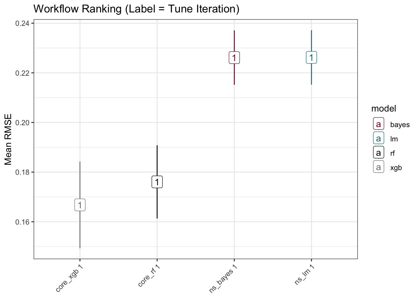

# --- Comment out for fit_resamples
# set_results |>
#   extract_workflow_set_result("core_rf") |> # core_xgb
#   unnest(.metrics) |>
#   summarise(.estimate = mean(.estimate), .config = first(.config),
#             .by = c(trees, mtry, min_n)) |> # tree_depth
#   arrange(.estimate) |>
#   slice_head(n = 1)
# ---------------------------------

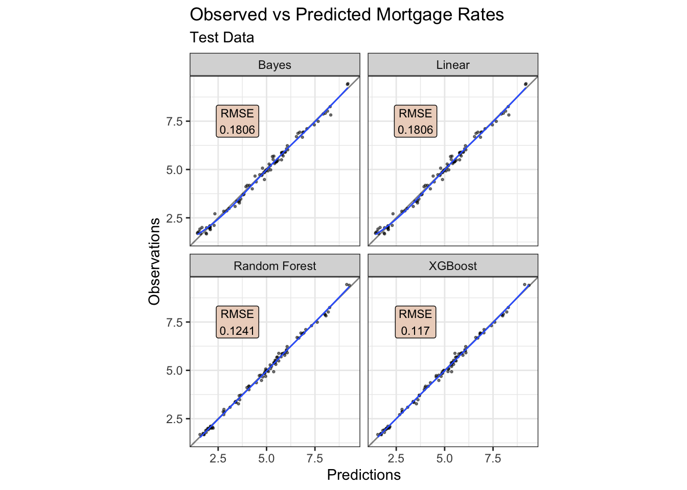
The models may then be assessed against the test data.

aug_train <- \(x){
  set.seed(2023)

  set_results |>
    filter(wflow_id == x) |>
    fit_best(metric = "rmse") |>
    augment(test)
}

walk2(
  c("xgb_res", "rf_res", "lm_res", "bayes_res"),
  c("core_xgb", "core_rf", "ns_lm", "ns_bayes"),
  \(x, y) assign(x, aug_train(y), .GlobalEnv)
)

The residuals from the trained model used on the test data look quite reasonable aside a small curvature pattern in the linear models. The presence of a pattern could suggest a missing explanatory variable(s), or non-linearity if present only in linear models.

focus_df <- bind_rows(
  rf = rf_res |> mutate(model = "Random Forest"),
  xgb = xgb_res |> mutate(model = "XGBoost"),
  lm = lm_res |> mutate(model = "Linear"),
  bayes = bayes_res |> mutate(model = "Bayes"),
  .id = "id"
)

label_df <- focus_df |>
  nest(-c(id, model)) |>
  mutate(metric = map(data, \(x) rmse(x, mortgage, .pred))) |>
  unnest(metric) |>
  mutate(mortgage = 7.5, .pred = 3.5, .estimate = round(.estimate, 4))

focus_df |>
  ggplot(aes(.pred, mortgage)) +
  geom_point(alpha = 0.5, size = 0.5) +
  geom_abline(alpha = 0.5) +
  geom_smooth(se = FALSE, size = 0.5) +
  geom_label(aes(label = glue("RMSE\n{.estimate}")),
    data = label_df, size = 3, fill = cols[2]
  ) +
  coord_obs_pred() +
  facet_wrap(~model) +
  labs(
    title = "Observed vs Predicted Mortgage Rates",
    subtitle = "Test Data",
    x = "Predictions", y = "Observations"
  )

focus_df |>
  mutate(residual = mortgage - .pred) |>
  ggplot(aes(sample = residual, colour = id)) +
  geom_qq() +
  geom_qq_line() +
  facet_wrap(~model) +
  scale_y_continuous(limits = c(-1, 1)) +
  scale_colour_manual(values = as.character(cols[c(1, 3, 5, 6)])) +
  labs(title = "QQ Plot of Residuals", subtitle = "Test Data")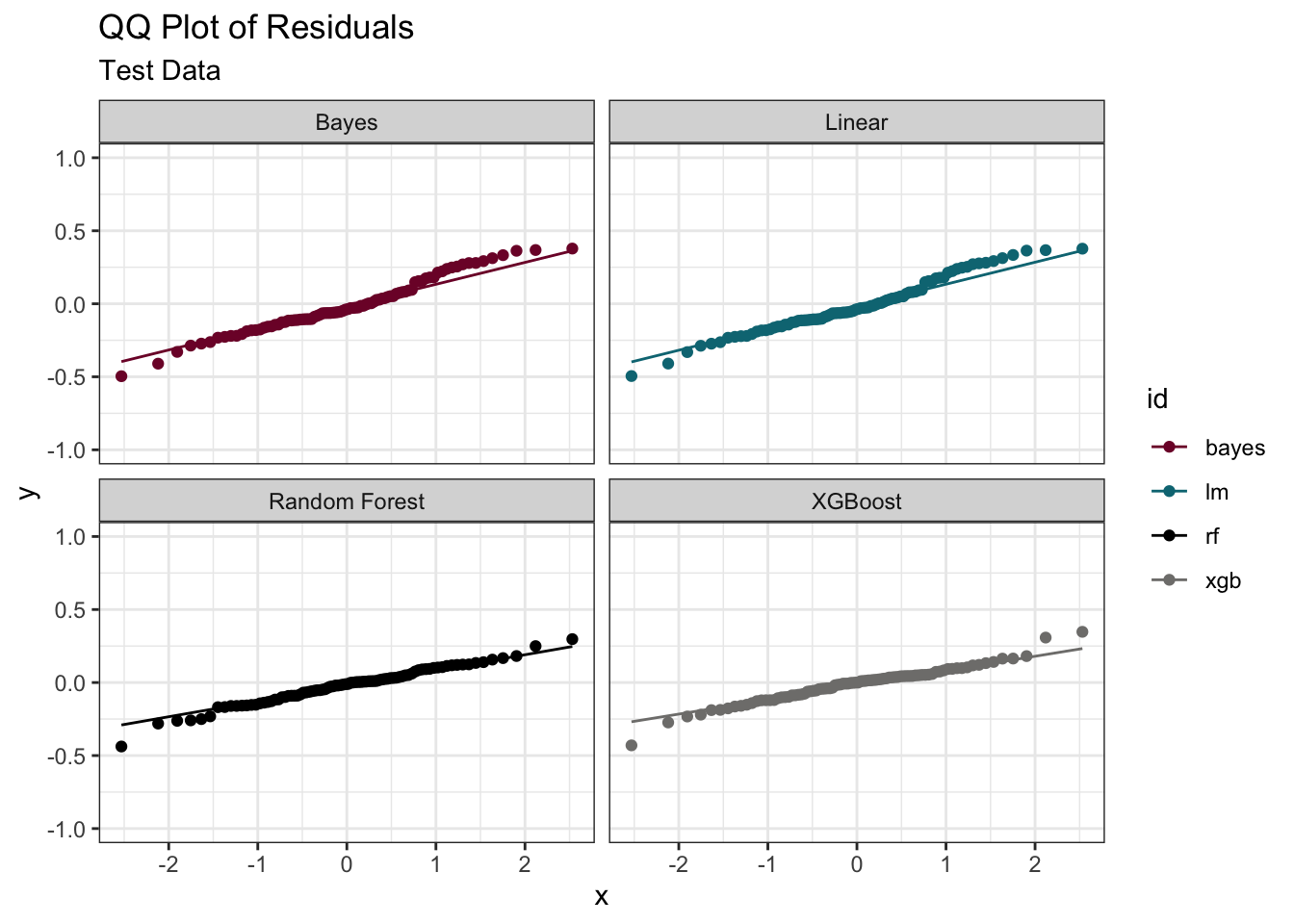

focus_df |>
  mutate(residual = mortgage - .pred) |>
  ggplot(aes(date, residual, colour = id)) +
  geom_hline(yintercept = 0, linetype = "dashed", colour = cols[3], linewidth = 1) +
  geom_point() +
  geom_smooth() +
  facet_wrap(~model) +
  scale_x_date(date_breaks = "2 years", date_labels = "%Y") +
  scale_y_continuous(limits = c(-1, 1)) +
  scale_colour_manual(values = as.character(cols[c(1, 3, 5, 6)])) +
  labs(title = "Residuals Over Time", subtitle = "Test Data", x = NULL, y = "Residuals") +
  theme(axis.text.x = element_text(angle = 45, hjust = 1))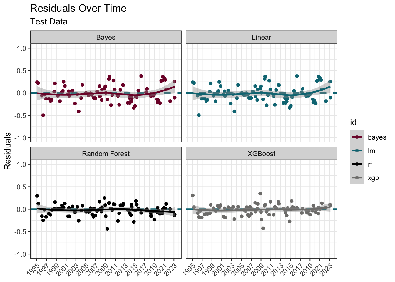

It makes sense to now train the tuned model(s) on all the historical data.

fit_hist <- \(y){
  set.seed(2023)

  model_set |>
    extract_workflow(y) |>
    fit(data = history_df)
}

walk2(
  c("xgb_fit", "rf_fit", "bayes_fit", "lm_fit"),
  c("core_xgb", "core_rf", "ns_bayes", "ns_lm"),
  \(x, y) assign(x, fit_hist(y), .GlobalEnv)
)

aug_fit <- \(y) y |> augment(forecast_df)

walk2(
  c("xgb_res", "rf_res", "bayes_res", "lm_res"),
  list(xgb_fit, rf_fit, bayes_fit, lm_fit),
  \(x, y) assign(x, aug_fit(y), .GlobalEnv)
)

Feature importance unsurprisingly confirms higher gilt and cbr values equate to higher mortgage rates.

set.seed(2023)

make_shap <- \(y){
  kernelshap(y,
    X = forecast_df,
    bg_X = train |> slice_sample(n = 50),
    feature_names = train |> select(-c(id, mortgage, mortgage_cut)) |> names(),
    parallel = TRUE
  ) |>
    shapviz()
}

tic()

walk2(
  c("xgb_shap", "rf_shap", "bayes_shap", "lm_shap"),
  list(xgb_fit, rf_fit, bayes_fit, lm_fit),
  \(x, y) assign(x, make_shap(y), .GlobalEnv)
)

toc()

mshap <- c(bayes = bayes_shap, xgb = xgb_shap, lm = lm_shap, rf = rf_shap)

# 119.9 sec elapsed

sv_importance(mshap, "beeswarm", color_bar_title = NULL) +
  plot_annotation(title = "Feature Importance (Yellow = High Feature Value)")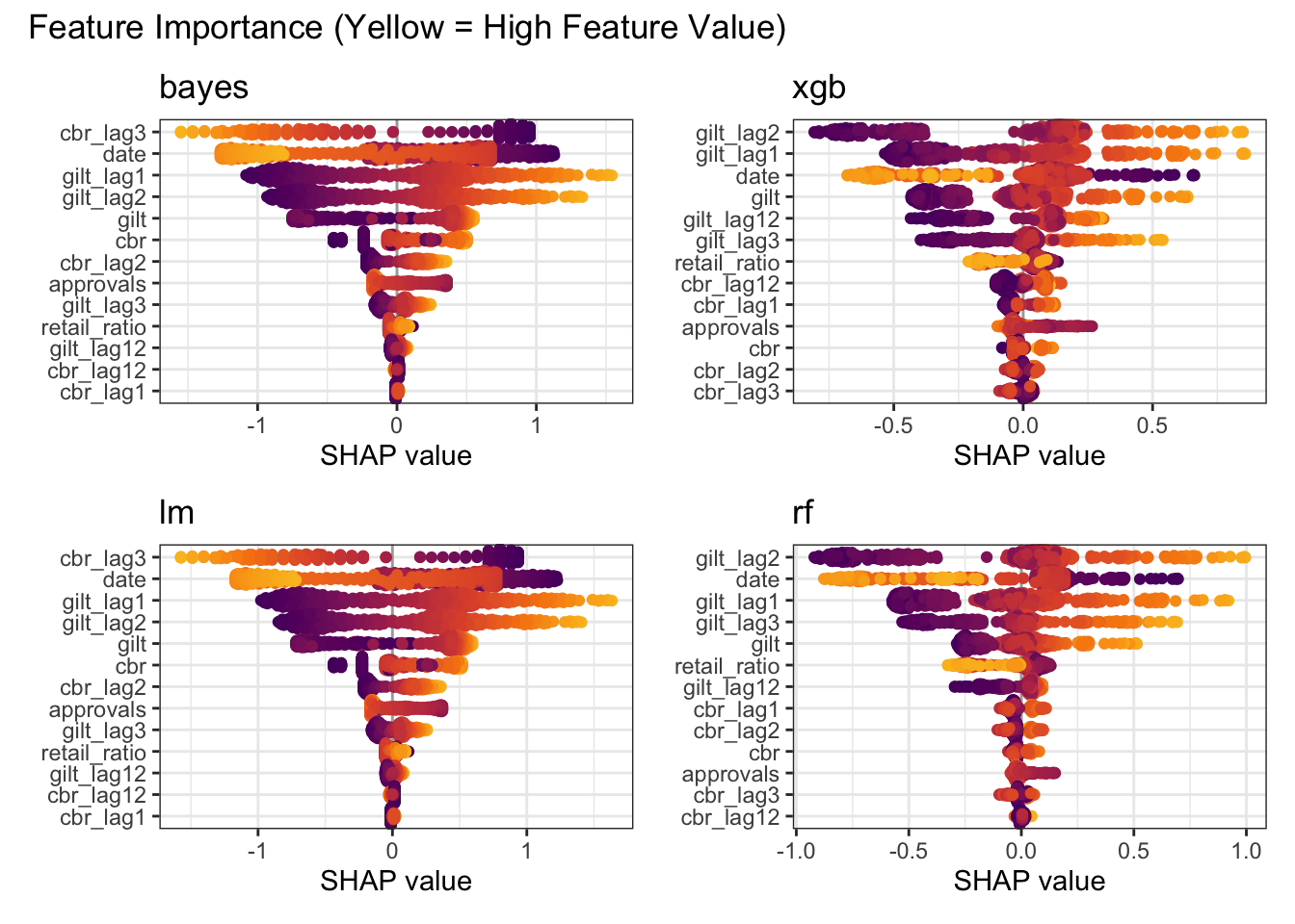

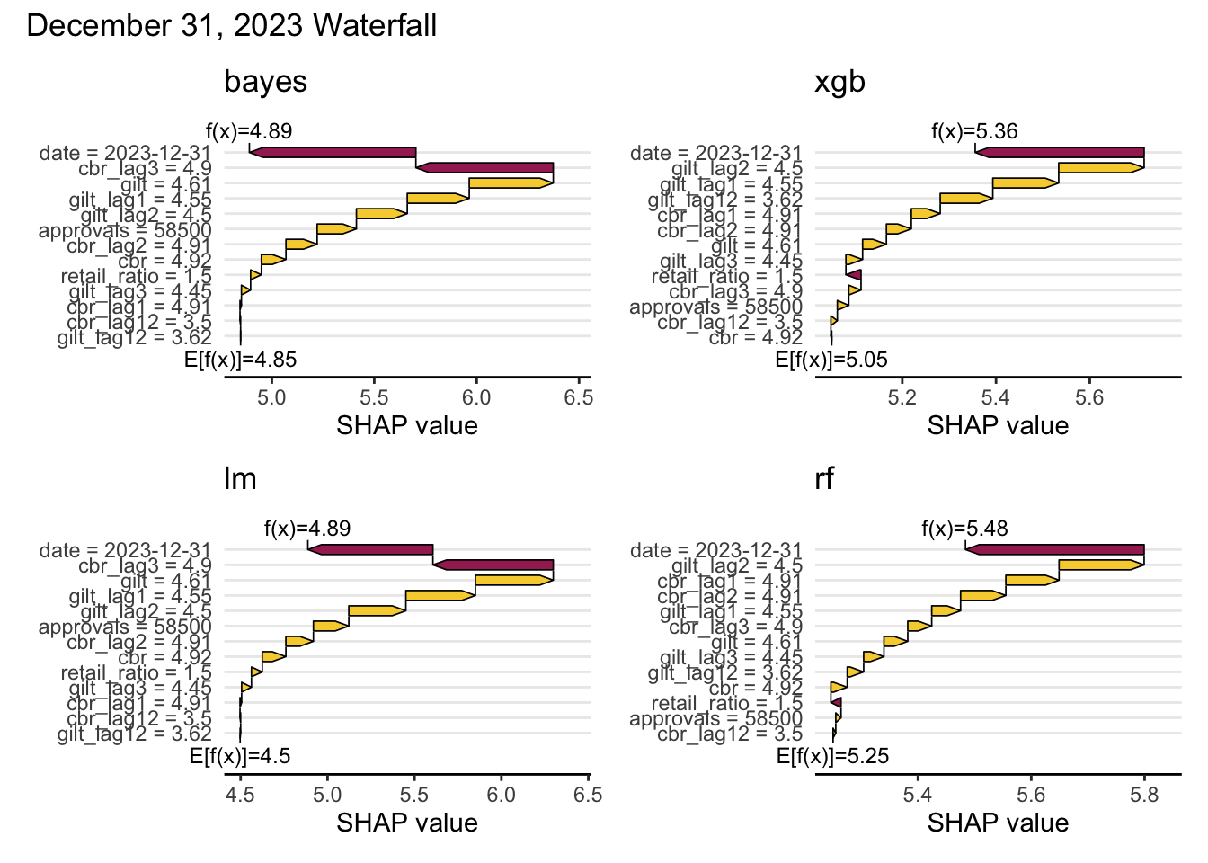
row_id <- last(which(forecast_df$date == max(forecast_df$date)))

sv_waterfall(mshap, row_id = row_id, max_display = 14) +
  plot_annotation(
    title = glue("{stamp('March 1, 2000')(max(forecast_df$date))} Waterfall")
  )

Whilst modelling with Bayesian (in contrast to linear) regression comes with the computational cost of Markov Chain Monte Carlo (MCMC) simulation, the pay-off is the provision of a credible range of values for each of the parameters in addition to the coefficient point estimates.

ci <- tidy(bayes_fit, conf.int = TRUE, conf.level = 0.9)

as.data.frame(extract_fit_engine(bayes_fit)) |>
  pivot_longer(everything(), names_to = "term") |>
  filter(term != "sigma") |>
  ggplot(aes(value)) +
  as_reference(geom_density(fill = "white"), id = "density") +
  with_blend(
    geom_rect(
      aes(
        x = NULL, y = NULL, xmin = conf.low, xmax = conf.high,
        ymin = -Inf, ymax = Inf, fill = term
      ),
      data = ci, colour = "grey50", fill = cols[1],
    ),
    bg_layer = "density", blend_type = "atop"
  ) +
  geom_vline(aes(xintercept = estimate),
    colour = "white",
    linetype = "dashed", data = ci
  ) +
  geom_density(colour = "grey50") +
  facet_wrap(~term, scales = "free") +
  labs(
    y = "Density", fill = "Term",
    title = "Bayesian Posterior Distributions", x = "Value",
    subtitle = "Terms with 90% Plausible Interval"
  ) +
  theme(legend.position = "none")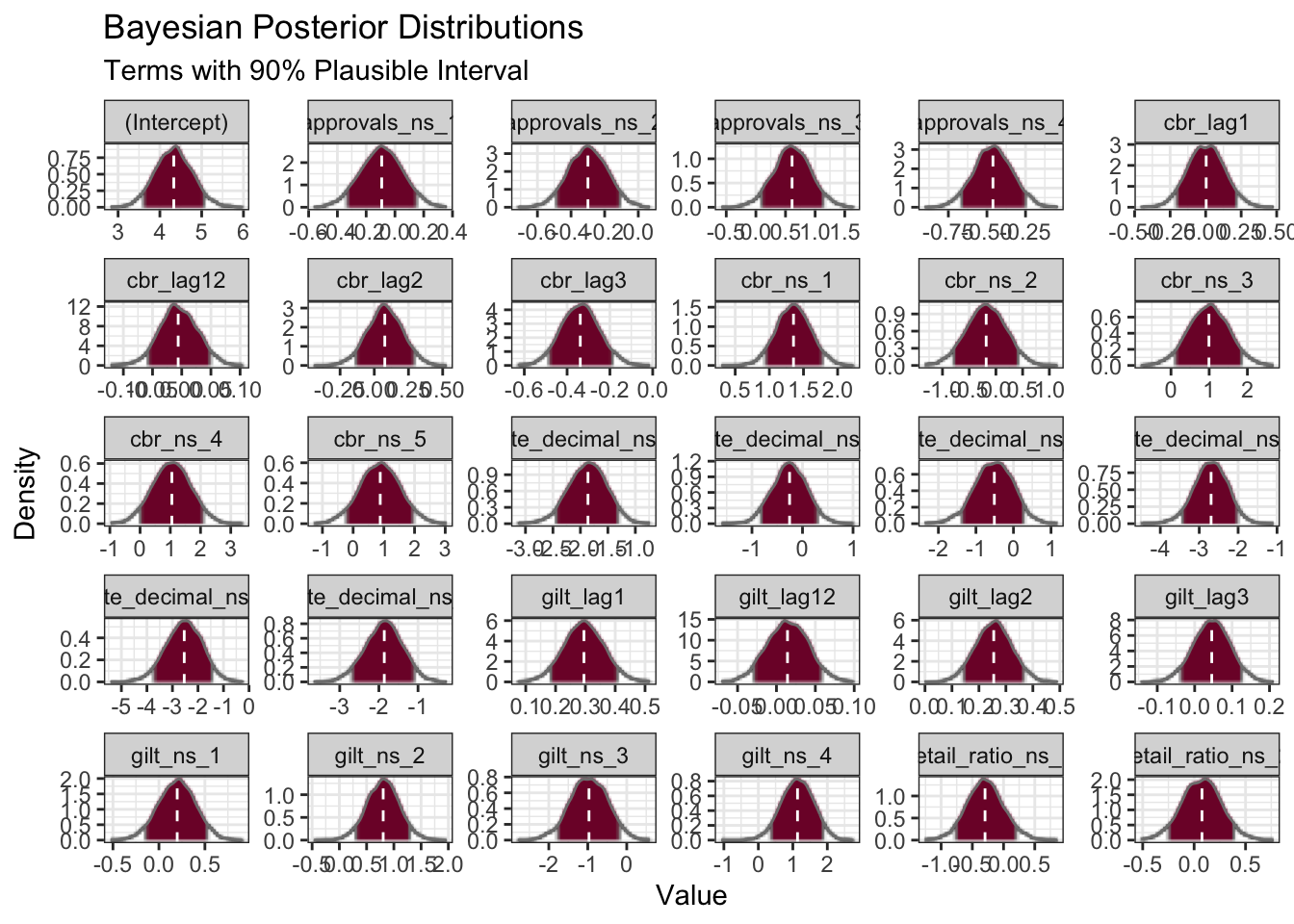

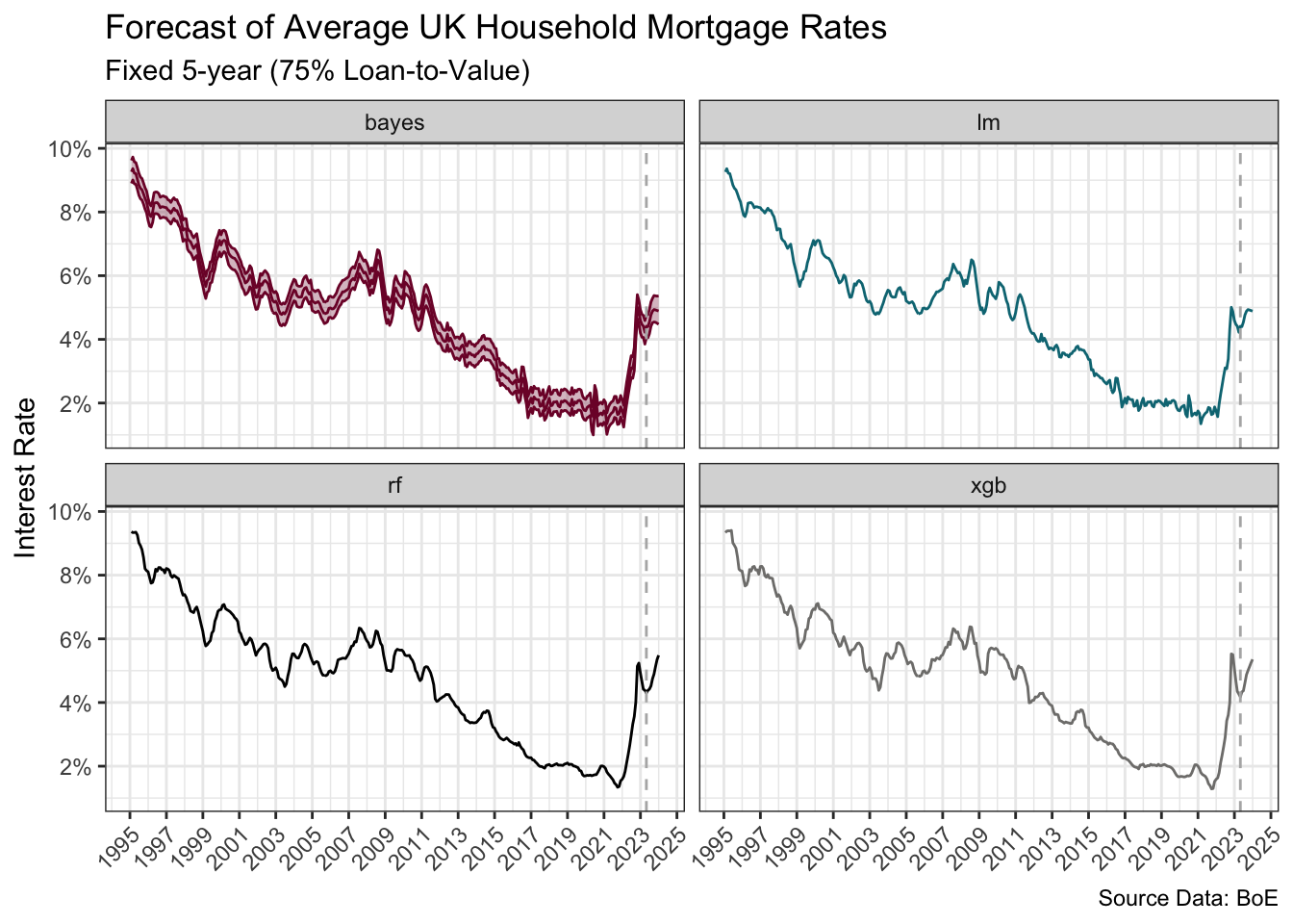
The plot below shows the final point estimate for each model as well as a 90% prediction interval for the Bayesian model using rstantools (Gabry et al. 2023).

The forecasts are, at least initially, directionally similar. The test residuals and RMSE would favour the non-linear models, and XGBoost in particular, over the linear models for these data. The forecasts are further dependent upon the quality of the forward-looking externally-sourced estimates for the predictors.

pi <- predictive_interval(extract_fit_engine(bayes_fit),
  newdata = ns_recipe |> prep() |> bake(new_data = forecast_df),
  prob = 0.9
) |>
  as_tibble() |>
  mutate(date = forecast_df$date)

bind_rows(
  xgb = xgb_res,
  bayes = bayes_res,
  rf = rf_res,
  lm = lm_res,
  .id = "model"
) |>
  left_join(pi, join_by(date)) |>
  mutate(across(c(`5%`, `95%`), \(x) if_else(model != "bayes", NA, x))) |>
  ggplot(aes(date, .pred, ymin = `5%`, ymax = `95%`, colour = model, fill = model)) +
  geom_ribbon(fill = cols[1], alpha = 0.3) +
  geom_line() +
  geom_vline(xintercept = ymd("2023-04-30"), linetype = "dashed", colour = "grey70") +
  scale_y_continuous(
    labels = label_number(suffix = "%"),
    breaks = c(2, 4, 6, 8, 10)
  ) +
  scale_x_date(date_breaks = "2 years", date_labels = "%Y") +
  scale_colour_manual(values = as.character(cols[c(1, 3, 5, 6)])) +
  scale_fill_manual(values = as.character(cols[c(1, 3, 5, 6)])) +
  labs(
    title = "Forecast of Average UK Household Mortgage Rates",
    subtitle = "Fixed 5-year (75% Loan-to-Value)",
    x = NULL, y = "Interest Rate",
    caption = "Source Data: BoE"
  ) +
  facet_wrap(~model) +
  theme(
    axis.text.x = element_text(angle = 45, hjust = 1),
    legend.position = "none"
  )

R Toolbox

Summarising below the packages and functions used in this post enables me to separately create a toolbox visualisation summarising the usage of packages and functions across all posts.

used_here()

Package	Function
base	as.character[7], as.data.frame[1], assign[5], c[27], library[21], list[7], max[2], names[1], readRDS[1], round[1], seq[1], set.seed[5], which[1]
conflicted	conflict_prefer_all[1], conflict_scout[1]
doParallel	registerDoParallel[1]
dplyr	across[3], arrange[1], bind_rows[3], distinct[1], filter[5], if_else[1], join_by[3], lag[3], last[2], left_join[2], mutate[18], nth[1], rename[1], rows_append[1], select[2], slice_head[1], slice_sample[1], tribble[1]
feasts	CCF[1]
forcats	fct_inorder[1], fct_reorder[1]
generics	augment[2], fit[1], tidy[1]
ggfx	as_reference[1], with_blend[1]
ggplot2	aes[14], annotate[1], autoplot[1], cut_number[1], element_blank[6], element_line[1], element_text[4], facet_wrap[5], geom_abline[1], geom_col[1], geom_density[2], geom_hline[1], geom_label[3], geom_line[2], geom_point[3], geom_pointrange[1], geom_qq[1], geom_qq_line[1], geom_rect[1], geom_ribbon[1], geom_smooth[3], geom_vline[3], ggplot[9], ggtitle[3], labs[16], position_dodge[1], scale_colour_manual[5], scale_fill_manual[2], scale_x_continuous[3], scale_x_date[3], scale_y_continuous[8], theme[10], theme_bw[3], theme_set[1], theme_void[1]
glue	glue[2]
hardhat	extract_fit_engine[2], extract_workflow[1]
janitor	clean_names[1]
kernelshap	kernelshap[1]
lubridate	dmy[1], floor_date[2], rollforward[1], stamp[1], year[1], ymd[7]
parsnip	boost_tree[1], linear_reg[2], rand_forest[1], set_engine[1]
patchwork	plot_annotation[4], plot_layout[2]
purrr	map[1], pwalk[1], reduce[1], walk2[4]
recipes	bake[1], has_role[1], prep[1], recipe[1], step_date[1], step_ns[4], update_role[3]
rsample	initial_split[1], testing[1], training[1], vfold_cv[1]
rstantools	predictive_interval[1]
rvest	html_element[1], html_table[1]
scales	cut_short_scale[1], label_number[8]
shapviz	shapviz[1], sv_importance[1], sv_waterfall[1]
stringr	str_c[2], str_extract[2]
tibble	as_tibble[1], tibble[2]
tictoc	tic[2], toc[2]
tidyr	nest[1], pivot_longer[1], unnest[1]
tidyselect	everything[1]
tsibble	as_tsibble[1], yearmonth[1]
tune	control_bayes[1], coord_obs_pred[1], fit_best[1]
usedthese	used_here[1]
workflowsets	rank_results[1], workflow_map[1], workflow_set[1]
xml2	read_html[1]
yardstick	metric_set[1], rmse[1]

References

Gabry, Jonah, Ben Goodrich, Martin Lysy, and Andrew Johnson. 2023. “Rstantools: Tools for Developing r Packages Interfacing with ’Stan’.” https://CRAN.R-project.org/package=rstantools.

Goodrich, Ben, Jonah Gabry, Imad Ali, and Sam Brilleman. 2023. “Rstanarm: Bayesian Applied Regression Modeling via Stan.” https://mc-stan.org/rstanarm/.

Kuhn, Max, and Simon Couch. 2023. “Workflowsets: Create a Collection of ’Tidymodels’ Workflows.” https://CRAN.R-project.org/package=workflowsets.

O’Hara-Wild, Mitchell, Rob Hyndman, and Earo Wang. 2023. “Fable: Forecasting Models for Tidy Time Series.” https://CRAN.R-project.org/package=fable.

Footnotes

Per Legal | Bank of England, the information made available via the Database is the copyright of the Governor and Company of the Bank, unless otherwise stated. Reproduction of data in the Database is subject to the terms of the UK Open Government Licence, allowing and encouraging free and flexible data reuse.↩︎
econforecasting.com (2023). Consensus Interest Rate Forecast Model. Retrieved from https://econforecasting.com/forecast-ukbankrate.↩︎
Estimated by Trading Economics ↩︎
Estimated by Trading Economics ↩︎
See Forecasting: Principles and Practice with implementation via the fable package(O’Hara-Wild, Hyndman, and Wang 2023).↩︎