Digging Deep

Do we see more planning applications when house sales are depressed?

In House Sales I looked at how a series of events damped down sales. By combining these sales data with planning applications I’d like to see if home owners “start digging” when they can’t sell.

Planning data is harvested with the kind permission of The Royal Borough of Kensington and Chelsea (RBKC). The code for these code chunks is not rendered out of courtesy to RBKC.

library(conflicted)
library(tidyverse)
conflict_prefer_all("dplyr", quiet = TRUE)
conflict_prefer("as_date", "lubridate")
library(rvest)
library(SPARQL)
library(quanteda)
library(quanteda.textstats)
library(wesanderson)
library(tictoc)
library(htmlwidgets)
library(clock)
library(fabletools)
library(feasts)
library(tsibble)
library(DT)
library(usedthese)

conflict_scout()

theme_set(theme_bw())

(cols <- wes_palette(name = "Darjeeling2"))

case_df <- readRDS("case.rds")

url <- 
  "https://www.freemaptools.com/download/full-postcodes/ukpostcodes.zip"

file_name <- basename(url)

url |> basename

download.file(url, file_name)

geocodes <- read_csv("ukpostcodes.zip")

The data need a bit of wrangling. And there is also the opportunity to try the newest column-wise enhancements to mutate: mutate_if and mutate_at have been superseded by mutate with across.

wide_df <- case_df |>
  pivot_wider(names_from = X1, values_from = X2) |>
  select(all_of(plan_colnames)) |>
  mutate(
    across(c(property_list, property_cons), \(vec) na_if(vec, "N/A")),
    across(c(app_comp, decision), \(vec) na_if(vec, ""))
  )

tidy_df <- wide_df |>
  mutate(
    dec_date = date_parse(dec_date, format = "%d %b %Y"),
    dec_year = get_year(dec_date),
    proposal_dev = str_to_lower(proposal_dev),
    property_pcode = str_extract(property_add, "SW10[\\s]?\\d[[:alpha:]]{2}"),
    property_pcode = str_replace(property_pcode, "SW10(?!\\s)", "SW10 "),
    app_comp = str_to_upper(app_comp) |>
      str_remove_all("[:punct:]") |>
      str_remove_all("\\b(?:AND|LTD|CO|LIMITED|UK|GROUP|LLP)\\b") |>
      str_squish(),
    decision = fct_explicit_na(decision, na_level = "Other"),
    decision = str_replace(decision, "/", " / "),
    dec_lump = fct_lump(decision, prop = 0.03),
    basement = if_else(str_detect(proposal_dev, "basement"), "Yes", "No"),
    property_listed = case_match(
      property_list,
      c("II", "II*", "2", "2*") ~ "Yes",
      .default = "No"
    ),
    app_comp = replace_na(app_comp, "None"),
    property_cons = if_else(property_cons == "" | is.na(property_cons),
      "None", property_cons
    ),
    proposal_dev = if_else(proposal_dev == "" | is.na(proposal_dev),
      "None", proposal_dev
    ),
    across(where(is.character), str_trim),
    across(c("app_comp", "proposal_type", "property_cons"), factor)
  ) |>
  left_join(geocodes, by = join_by(property_pcode == postcode))

tidy_df |>
  count(dec_lump) |>
  arrange(desc(n)) |>
  rename("Decision" = dec_lump, "Count" = n)

Decision	Count
Grant Planning Permission / Consent	5336
Withdrawn by Applicant	1123
Other	847
Refuse Planning Permission / Consent	752
Discharge of Conditions - Grant	626
Raise No Objection	418

quanteda (Benoit et al. 2018) to look at key words in context (kwic).

I’d like to review planning applications by theme. So I’ll first need to get a sense of what the themes are by plotting the words which appear most frequently.

plus_words <-
  c("new",
    "pp",
    "two",
    "one",
    "dated",
    "withdrawn",
    "flat",
    "x",
    "permission",
    "rear",
    "first",
    "second",
    "planning",
    "floor",
    "erection"
  )

words <- tidy_df |> 
  corpus(text_field = "proposal_dev", 
         doc_vars = c("dec_date", "proposal_type", 
                      "decision", "dec_year")) |> 
  dfm(
    remove = c(stopwords("english"), plus_words),
    remove_numbers = TRUE,
    remove_punct = TRUE) |> 
  textstat_frequency() |> 
  slice_head(n = 30) |> 
  mutate(feature = fct_reorder(feature, frequency))

words |> 
  ggplot(aes(feature, frequency)) +
  geom_col(fill = cols[4]) +
  coord_flip() +
  labs(x = NULL, y = NULL, 
       title = "Frequent Planning Proposal Words",
       caption = "Source: RBKC Planning Search")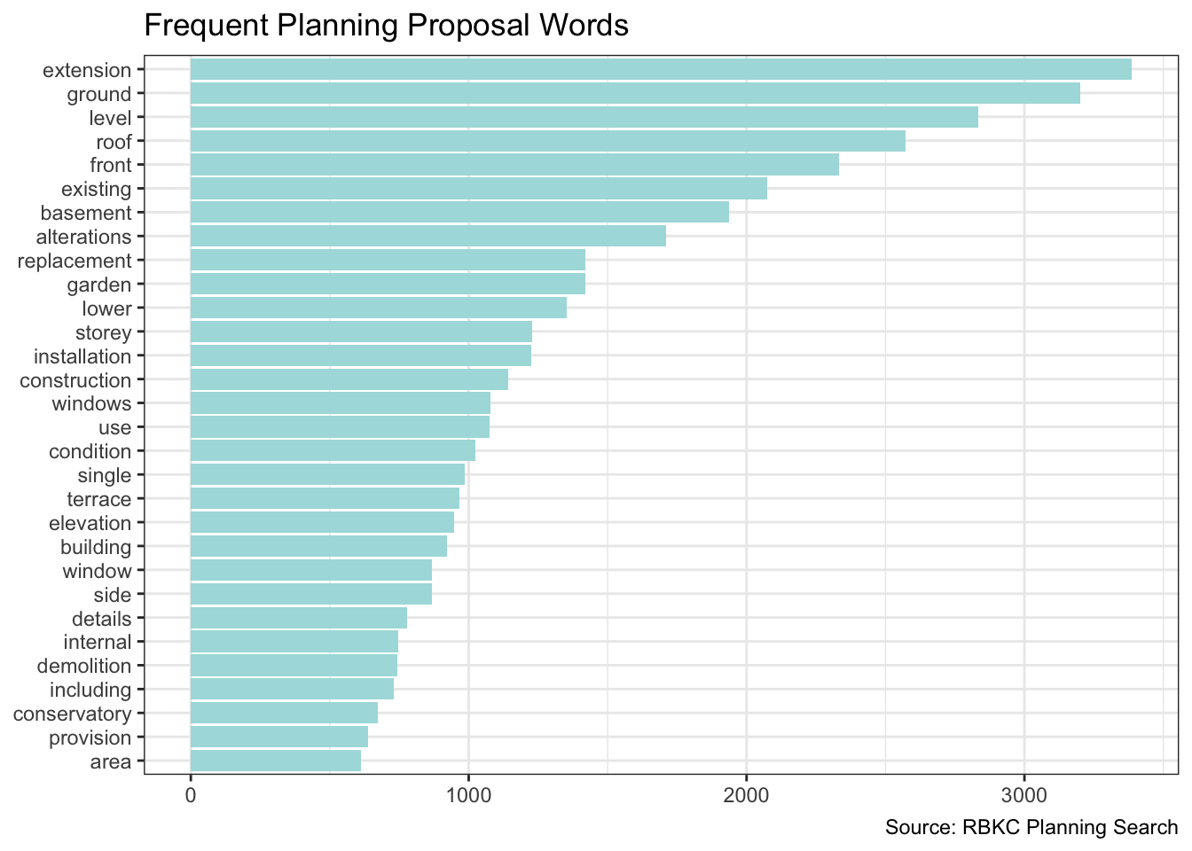

Now I can create a theme feature.

remapped_df <- tidy_df |>
  mutate(
    theme = case_when(
      str_detect(proposal_dev, "basem|excav") ~ "Basement or Excavation",
      str_detect(proposal_dev, "xten|vatory|torey") ~ "Extension, Conservatory \nor Storey",
      str_detect(proposal_dev, "windo|doo") ~ "Windows or Doors",
      str_detect(proposal_dev, "roof") ~ "Roof",
      str_detect(proposal_dev, "rrac|dsc|garde") | 
        str_detect(proposal_type, "Tree") ~ "Trees, Landscaping, \nGarden or Terrace",
      .default = "Other"
    ),
    outcome = case_when(
      str_detect(decision, "Gran|No Ob|Accep|Lawf") ~ "Positive",
      str_detect(decision, "Refus") ~ "Refuse",
      str_detect(decision, "Withdr") ~ "Withdrawn",
      .default = "Other"
    )
  )

I also want to compare house sales with planning applications over time. So, I’ll re-use the SPARQL query from House Sales.

tic()

endpoint <- "https://landregistry.data.gov.uk/landregistry/query"

query <- 'PREFIX  text: <http://jena.apache.org/text#>
PREFIX  ppd:  <http://landregistry.data.gov.uk/def/ppi/>
PREFIX  lrcommon: <http://landregistry.data.gov.uk/def/common/>
  
SELECT  ?item ?ppd_propertyAddress ?ppd_hasTransaction ?ppd_pricePaid ?ppd_transactionCategory ?ppd_transactionDate ?ppd_transactionId ?ppd_estateType ?ppd_newBuild ?ppd_propertyAddressCounty ?ppd_propertyAddressDistrict ?ppd_propertyAddressLocality ?ppd_propertyAddressPaon ?ppd_propertyAddressPostcode ?ppd_propertyAddressSaon ?ppd_propertyAddressStreet ?ppd_propertyAddressTown ?ppd_propertyType ?ppd_recordStatus

WHERE
{ ?ppd_propertyAddress text:query _:b0 .
  _:b0 <http://www.w3.org/1999/02/22-rdf-syntax-ns#first> lrcommon:postcode .
  _:b0 <http://www.w3.org/1999/02/22-rdf-syntax-ns#rest> _:b1 .
  _:b1 <http://www.w3.org/1999/02/22-rdf-syntax-ns#first> "( SW10 )" .
  _:b1 <http://www.w3.org/1999/02/22-rdf-syntax-ns#rest> _:b2 .
  _:b2 <http://www.w3.org/1999/02/22-rdf-syntax-ns#first> 3000000 .
  _:b2 <http://www.w3.org/1999/02/22-rdf-syntax-ns#rest> <http://www.w3.org/1999/02/22-rdf-syntax-ns#nil> .
  ?item ppd:propertyAddress ?ppd_propertyAddress .
  ?item ppd:hasTransaction ?ppd_hasTransaction .
  ?item ppd:pricePaid ?ppd_pricePaid .
  ?item ppd:transactionCategory ?ppd_transactionCategory .
  ?item ppd:transactionDate ?ppd_transactionDate .
  ?item ppd:transactionId ?ppd_transactionId
  
  OPTIONAL { ?item ppd:estateType ?ppd_estateType }
  OPTIONAL { ?item ppd:newBuild ?ppd_newBuild }
  OPTIONAL { ?ppd_propertyAddress lrcommon:county ?ppd_propertyAddressCounty }
  OPTIONAL { ?ppd_propertyAddress lrcommon:district ?ppd_propertyAddressDistrict }
  OPTIONAL { ?ppd_propertyAddress lrcommon:locality ?ppd_propertyAddressLocality }
  OPTIONAL { ?ppd_propertyAddress lrcommon:paon ?ppd_propertyAddressPaon }
  OPTIONAL { ?ppd_propertyAddress lrcommon:postcode ?ppd_propertyAddressPostcode }
  OPTIONAL { ?ppd_propertyAddress lrcommon:saon ?ppd_propertyAddressSaon }
  OPTIONAL { ?ppd_propertyAddress lrcommon:street ?ppd_propertyAddressStreet }
  OPTIONAL { ?ppd_propertyAddress lrcommon:town ?ppd_propertyAddressTown }
  OPTIONAL { ?item ppd:propertyType ?ppd_propertyType }
  OPTIONAL { ?item ppd:recordStatus ?ppd_recordStatus }
}'

sales <- SPARQL(endpoint, query)

toc()

196.543 sec elapsed

Let’s now bind the data into one tibble and summarise the transaction volumes over time.

sales_df <- sales$results |> 
  as_tibble() |>
  mutate(
    date = as_datetime(ppd_transactionDate) |> as_date(),
    dataset = "Sales"
  ) |>
  summarise(volume = n(), .by = c(date, dataset))

app_df <- remapped_df |>
  mutate(
    date = dec_date,
    dataset = "Planning"
  ) |>
  summarise(volume = n(), .by = c(date, dataset))

compare_df <- bind_rows(app_df, sales_df)

summary_df <- compare_df |>
  filter(date >= min(sales_df$date)) |> 
  mutate(date = date_build(get_year(date), get_month(date), "last")) |> 
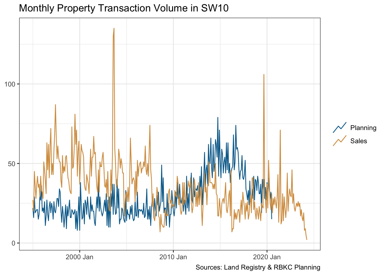
  summarise(volume = sum(volume), .by = c(date, dataset))

The visualisation below does suggest that home owners “start digging” when they can’t sell. At least in this part of London.

monthly_ts <- summary_df |> 
  mutate(date = yearmonth(date)) |> 
  as_tsibble(key = dataset, index = date)

monthly_ts |> 
  ggplot(aes(date, volume, colour = dataset)) +
  geom_line(key_glyph = "timeseries") +
  scale_colour_manual(values = cols[c(2, 3)]) +
  labs(x = NULL, y = NULL, colour = NULL,
       title = "Monthly Property Transaction Volume in SW10",
       caption = "Sources: Land Registry & RBKC Planning"
       )

Time-series data may have an underlying trend and a seasonality pattern. I’ll use the seasonal package to decompose each time-series. Each exhibit annual seasonality which evolves over time.

monthly_ts |>
  model(stl = STL(volume ~ season())) |>
  components() |> 
  autoplot() +
  scale_colour_manual(values = cols[c(2, 3)]) +
  labs(x = NULL, title = "Time Series Decomposition")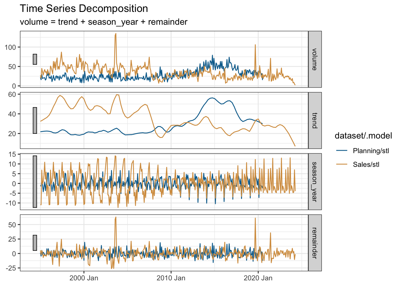

We also see some inverse correlation between the two time-series re-affirming the visual conclusion that planning applications increase when the housing market is depressed.

monthly_ts |> 
  pivot_wider(names_from = dataset, values_from = volume) |>
  CCF(Sales, Planning, lag_max = 6) |> 
  autoplot() +
  labs(title = "Correlation Between Sales & Planning") +
  theme(axis.text.x = element_text(angle = 45, hjust = 1))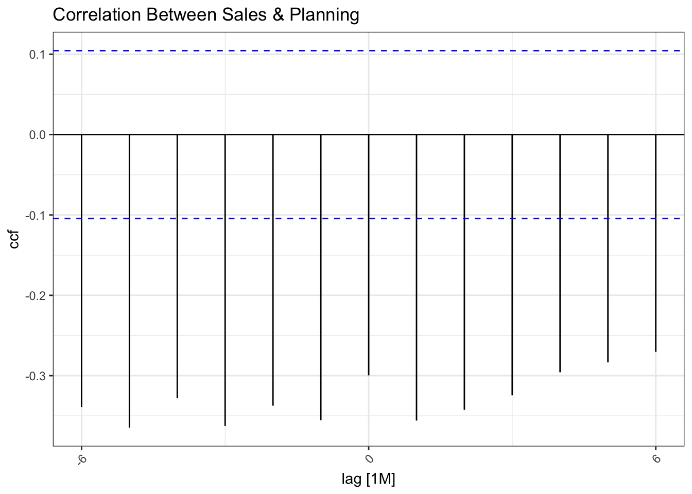

The overall volumes of planning applications and house transactions in SW10 are fairly similar.

summary_df |>
  summarise(total = sum(volume), .by = dataset) |> 
  rename("Dataset" = dataset, "Count" = total)

Dataset	Count
Planning	8926
Sales	11764

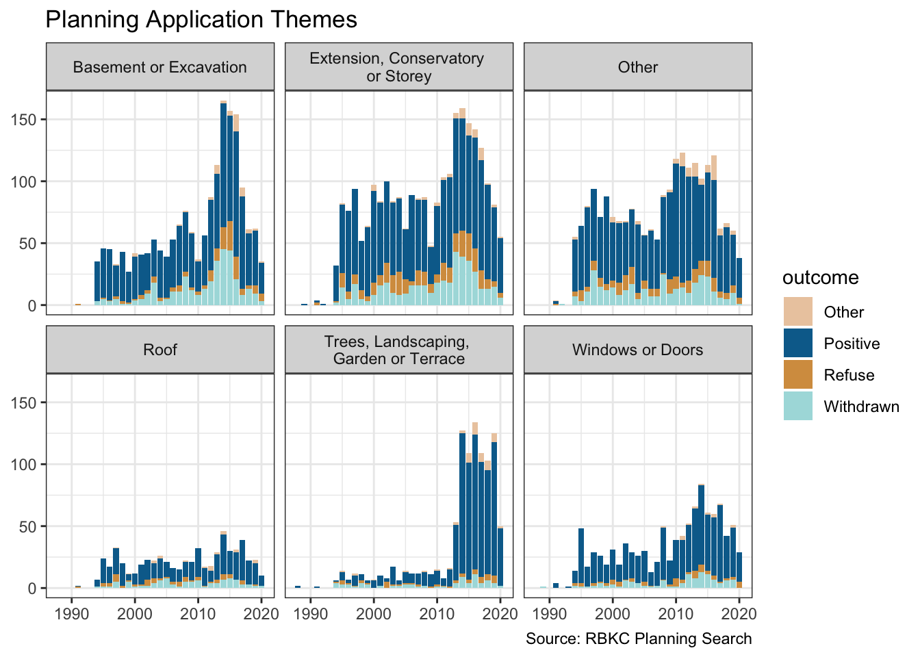
Earlier, I added a “theme” feature to the data. So let’s take a look at the volume of applications over time faceted by theme and coloured by the outcome. We see that the rise in planning applications is fuelled by basements or excavations, and work on outside landscaping and terracing. So perhaps we do “dig” when we can’t sell.

remapped_df |>
  ggplot(aes(dec_year, fill = outcome)) +
  geom_bar() +
  facet_wrap( ~ theme, nrow = 2) +
  scale_fill_manual(values = cols[c(1:4)]) +
  labs(
    title = "Planning Application Themes",
    x = NULL, y = NULL,
    caption = "Source: RBKC Planning Search"
    )

R Toolbox

Summarising below the packages and functions used in this post enables me to separately create a toolbox visualisation summarising the usage of packages and functions across all posts.

used_here()

Package	Function
DT	datatable[1]
SPARQL	SPARQL[1]
base	as.numeric[1], basename[1], c[16], is.na[2], library[15], min[1], readRDS[1], saveRDS[1], sum[2]
clock	date_build[1], date_parse[1], get_month[1], get_year[2]
conflicted	conflict_prefer[1], conflict_prefer_all[1], conflict_scout[1]
dplyr	across[4], arrange[1], bind_rows[2], case_match[1], case_when[2], count[1], desc[1], filter[2], if_else[3], join_by[1], left_join[1], mutate[9], n[2], na_if[2], rename[2], select[2], slice_head[1], summarise[4]
fabletools	components[1], model[1]
feasts	CCF[1], STL[1]
forcats	fct_explicit_na[1], fct_lump[1], fct_reorder[1]
ggplot2	aes[3], autoplot[2], coord_flip[1], element_text[1], facet_wrap[1], geom_bar[1], geom_col[1], geom_line[1], ggplot[3], labs[5], scale_colour_manual[2], scale_fill_manual[1], theme[1], theme_bw[1], theme_set[1]
htmlwidgets	saveWidget[1]
lubridate	as_date[1], as_datetime[1]
purrr	list_rbind[2], map[2]
quanteda	corpus[2], dfm[1], kwic[1], phrase[1]
quanteda.textstats	textstat_frequency[1]
readr	read_csv[1]
rvest	html_attr[1], html_element[2], html_elements[2], html_table[1], html_text[1]
stopwords	stopwords[1]
stringr	str_c[3], str_detect[11], str_extract[1], str_remove_all[2], str_replace[2], str_squish[1], str_to_lower[1], str_to_upper[1]
tibble	as_tibble[2], tibble[1]
tictoc	tic[2], toc[2]
tidyr	pivot_wider[2], replace_na[1]
tidyselect	all_of[1], where[1]
tsibble	as_tsibble[1], yearmonth[1]
usedthese	used_here[1]
utils	download.file[1]
wesanderson	wes_palette[1]
xml2	read_html[3]

References

Benoit, Kenneth, Kohei Watanabe, Haiyan Wang, Paul Nulty, Adam Obeng, Stefan Müller, and Akitaka Matsuo. 2018. “Quanteda: An r Package for the Quantitative Analysis of Textual Data” 3: 774. https://doi.org/10.21105/joss.00774.