Seeing the Wood for the Trees

Visualising small multiples when crime data leave you unable to see the wood for the trees

In Criminal Goings-on faceting offered a way to get a sense of the data. This is a great visualisation tool building on the principle of small multiples. There may come a point though where the sheer volume of small multiples make it harder to “see the wood for the trees”. What’s an alternative strategy?

library(conflicted)
library(tidyverse)
conflict_prefer_all("dplyr", quiet = TRUE)
library(trelliscope)
library(janitor)
library(vangogh)
library(usedthese)

conflict_scout()

This time I’ll use Van Gogh’s “The Starry Night” palette for the feature image and plots. And there are 12 types of criminal offence, so colorRampPalette will enable the interpolation of an extended set.

theme_set(theme_bw())

(cols <- vangogh_palette("StarryNight"))

cols12 <- colorRampPalette(cols)(12)

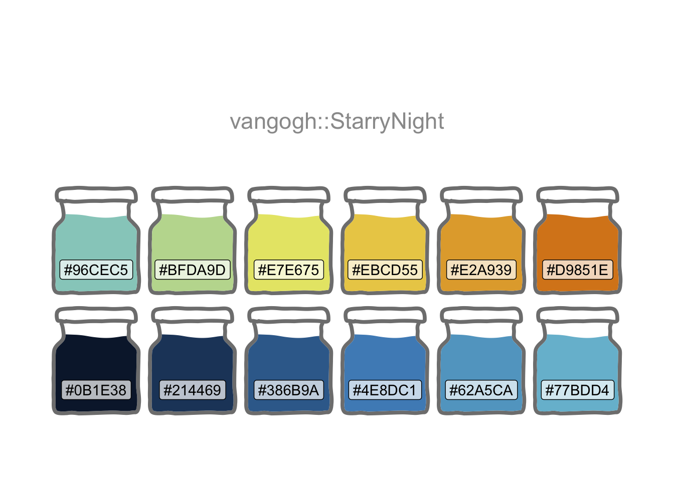
The data need a little tidy-up.

crime_df <- str_c(
  "https://data.london.gov.uk/download/recorded_crime_summary/",
  "934f2ddb-5804-4c6a-a17c-bdd79b33430e/", 
  "MPS%20Borough%20Level%20Crime%20%28Historical%29.csv"
  ) |> 
  read_csv(show_col_types = FALSE) |> 
  clean_names() |> 
  rename_with(\(x) str_remove_all(x, "_text|look_up_|_name")) |> 
  pivot_longer(where(is.numeric), names_to = "month", values_to = "num_offences") |> 
  mutate(month = parse_number(month) |> str_c("01") |> ymd())

The original visualisation in Criminal Goings-on using ggplot’s facet_wrap is a little tricky to digest, even when limited to major categories of crime.

crime_df |>
  summarise(num_offences = sum(num_offences), .by = c(major, borough, month)) |>
  ggplot(aes(month, num_offences, colour = major, group = major)) +
  geom_line() +
  facet_wrap(~borough, scales = "free_y", ncol = 4) +
  labs(
    x = NULL, y = NULL, title = "London Crime by Borough",
    colour = "Offence", caption = "Source: data.gov.uk"
  ) +
  scale_colour_manual(values = cols12) +
  guides(colour = guide_legend(nrow = 3)) +
  theme(
    strip.background = element_rect(fill = cols[4]),
    legend.position = "bottom",
    axis.text.x = element_text(angle = 45, hjust = 1)
  ) + 
  guides(col = guide_legend(ncol = 2))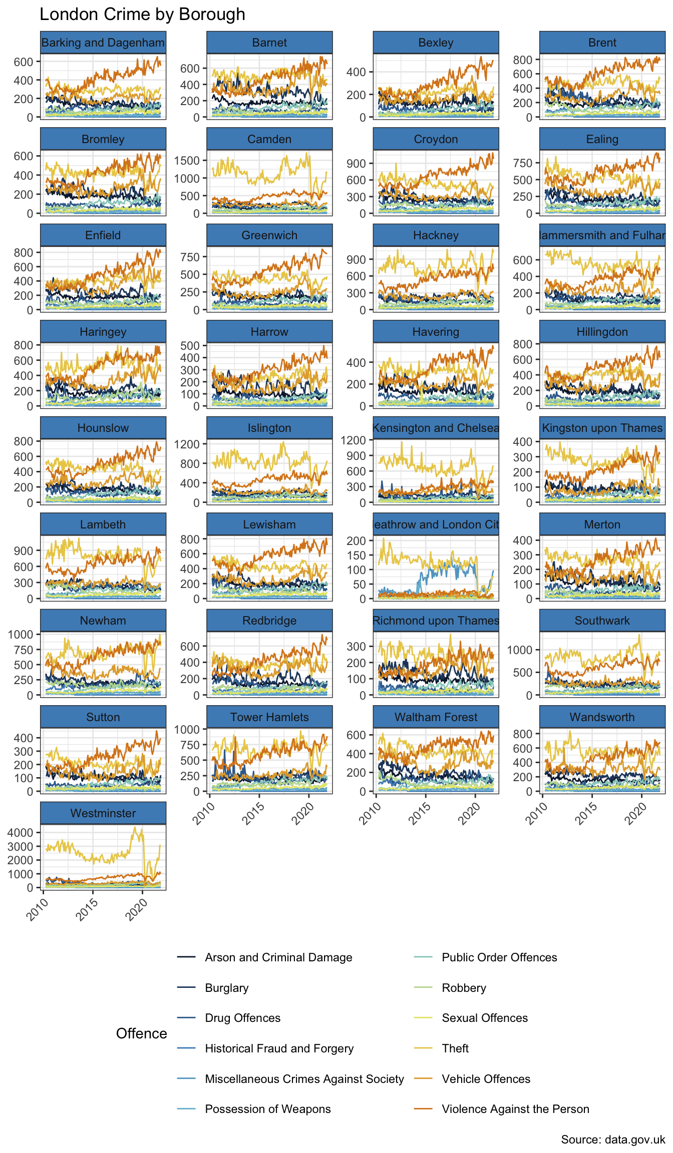

This “little project” was first published using trelliscopejs which offered a really nice alternative approach to the static facet_wrap. This has been recently reimagined by the superior and easier-to-use trelliscope package. I’ve updated this post to use the “latest and greatest”.

Click top-right to pop the display out full screen. Over 1,700 time series plots may be interactively filtered and sorted (for every combination of borough, major/minor category of crime) using summary statistics such as the steepness of the linear trend line.

panels_df <- crime_df |>
  mutate(major = str_wrap(major, 16)) |> 
  ggplot(aes(month, num_offences)) +
  geom_line(show.legend = FALSE) +
  geom_smooth(method = "lm", se = FALSE, colour = cols[5]) +
  facet_panels(vars(borough, major, minor), scales = "free") + 
  labs(colour = NULL, x = NULL, y = "Offence Count")

slope <- \(x, y) coef(lm(y ~ x))[2]

summary_df <- crime_df |> 
  summarise(
    mean_count = mean(num_offences), 
    slope = slope(month, num_offences),
    .by = c(borough, major, minor))
  
panels_df |>
  as_panels_df(as_plotly = TRUE) |>
  as_trelliscope_df(
    name = "Crime in 'The Smoke'",
    description = str_c(
      "Timeseries of offences by category ",
      "across London's 33 boroughs sourced from data.gov.uk."
    )
  ) |>
  left_join(summary_df, join_by(borough, major, minor)) |>
  set_var_labels(
    major = "Major Category of Offence",
    minor = "Minor Category of Offence",
    mean_count = "Average Offences by Borough & Offence Category",
    slope = "Steepness of a Linear Trendline"
  ) |>
  set_default_sort(c("slope"), dirs = "desc") |>
  set_tags(
    stats = c("mean_count", "slope"),
    info = c("borough", "major", "minor")
  ) |>
  set_theme(
    primary = cols[1],
    dark = cols[1],
    light = cols[5],
    light_text_on_dark = TRUE,
    dark_text = cols[1],
    light_text = cols[4],
    header_background = cols[2],
    header_text = NULL
  ) |>
  view_trelliscope()

R Toolbox

Summarising below the packages and functions used in this post enables me to separately create a toolbox visualisation summarising the usage of packages and functions across all posts.

used_here()

Package	Function
base	c[5], library[6], mean[1], sum[1]
conflicted	conflict_prefer_all[1], conflict_scout[1]
dplyr	join_by[1], left_join[1], mutate[2], rename_with[1], summarise[2], vars[1]
ggplot2	aes[2], element_rect[1], element_text[1], facet_wrap[1], geom_line[2], geom_smooth[1], ggplot[2], guide_legend[2], guides[2], labs[2], scale_colour_manual[1], theme[1], theme_bw[1], theme_set[1]
grDevices	colorRampPalette[1]
janitor	clean_names[1]
lubridate	ymd[1]
readr	parse_number[1], read_csv[1]
stats	coef[1], lm[1]
stringr	str_c[3], str_remove_all[1], str_wrap[1]
tidyr	pivot_longer[1]
tidyselect	where[1]
trelliscope	as_panels_df[1], as_trelliscope_df[1], facet_panels[1], set_default_sort[1], set_tags[1], set_theme[1], set_var_labels[1], view_trelliscope[1]
usedthese	used_here[1]
vangogh	vangogh_palette[1]